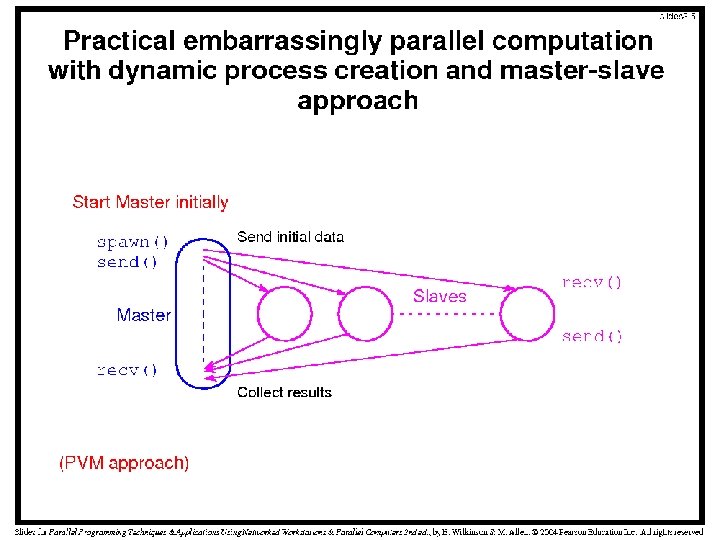
Characteristics of Embarrassingly Parallel Computations Easily parallelizable Little
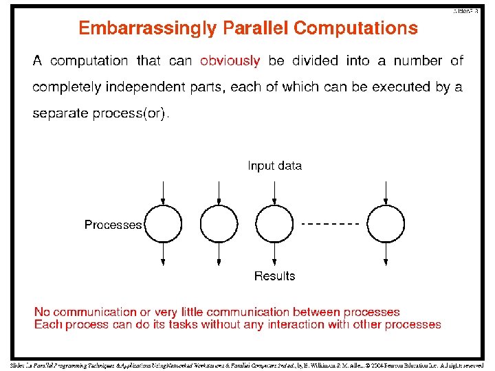

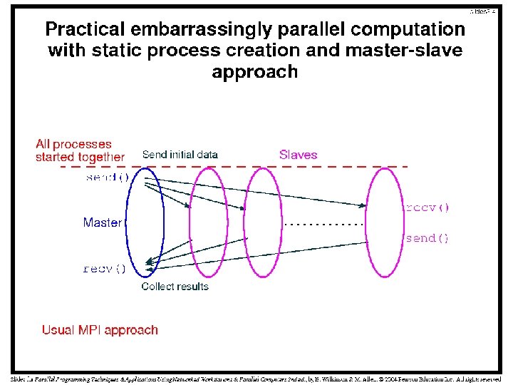
Characteristics of Embarrassingly Parallel Computations • Easily parallelizable • Little or no interaction between processes • Can give maximum speedup if all available processors are kept busy • The only constructs required are simply to distribute the data and to start the processes • Since the data is not shared, message-passing multicomputers are appropriate for such computations


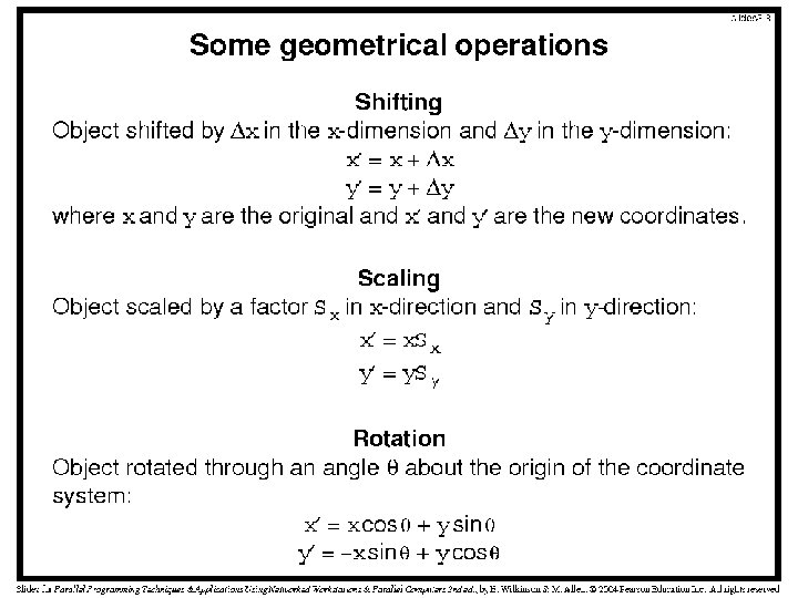
Representation of Images • The most basic way to store a two-dimensional image is a pixmap, in which each pixel is stored as a binary number in a two-dimensional array. – black-and-white - 1 bit per pixel – greyscale - 8 bits per pixel – color - 24 bits (RGB) • Geometrical transformations require mathematical operations performed on pixels coordinates – Transformations move a pixel’s position without affecting its value. – Transformations must be done at high speed to be acceptable • Pixels transformations are independent – Truly embarrassingly parallel computations

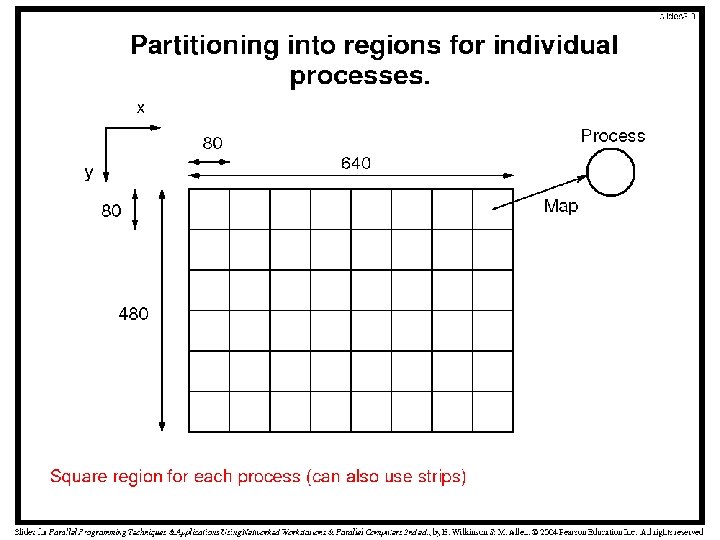
Parallel Programming Concern • The input data is the bitmap typically held in a file copied into an array • Main parallel programming concern: division of bitmap into group of pixels for each process – Typically more pixels than processors • Two general methods of grouping – By square/rectangular region – By columns/rows • Example: A 640 x 480 image, 48 processes – Divide display area into 48 80 x 80 square areas – Divide display area into 48 rows of 640 x 10 pixels • This method of division appears in applications involving processing 2 -D data

Partition into Rows: Master Process for (i = 0, row = 0; i < 48; i++, row = row + 10) send(row, P[i]); for (i = 0; i < 480; i++) for (j = 0; j < 640; j++) temp_map[i][j] = 0; for (i = 0; i < (640 * 480); i++) { recv(oldrow, oldcol, newrow, newcol, P[ANY]); if (!((newrow < 0)||(newrow >= 480)|| (newcol < 0)||(newcol >= 640))) temp_map[newrow][newcol] = map[oldrow][oldcol]; } for (i = 0; i < 480; i++) for (j = 0; j < 640; j++) map[i][j] = temp_map[i][j];
![Slave Processes recv(row, P[MASTER]); for (oldrow = row; oldrow < (row + 10); oldrow++)](http://slidetodoc.com/presentation_image_h2/2608f735f28e86314560657198badb3c/image-14.jpg "Slave Processes recv(row, P[MASTER]); for (oldrow = row; oldrow < (row + 10); oldrow++)")
Slave Processes recv(row, P[MASTER]); for (oldrow = row; oldrow < (row + 10); oldrow++) for (oldcol = 0; oldcol < 640; oldcol++) { newrow = oldrow + delta_x; newcol = oldcol + delta_y; send(oldrow, oldcol, newrow, newcol, P[MASTER]); }

Program Analysis • Suppose each pixel requires two computational steps and there are n x n pixels. – ts = 2 n 2 - (O(n 2)) • Communication: – p processes – Before the computation, the starting row numbers must be sent to each process. – The individual processes have to send back the transformed coordinates of their group of pixels. – tcomm = p(tstartup +tdata)+n 2(tstartup +4 tdata) = O(p+n 2) • Computation: – Groups of n 2/p. – Each pixel requires 2 additions. – tcomp = 2(n 2/p) = O(n 2/p) • For fixed p, the time complexity is O(n 2).

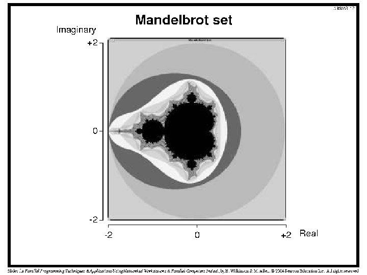
Mandelbrot Set • The Mandelbrot set is a widely used test in parallel computer systems – It is computationally intensive • Displaying this set is another example of processing a bit-mapped image • In contrast to the previous example, the image is computed in this case
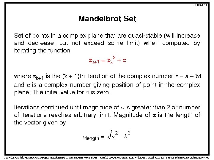
 • Computing the function zk+1=zk 2+c, is simplified by recognizing that")
Mandelbrot Set (cont’d) • Computing the function zk+1=zk 2+c, is simplified by recognizing that – z 2 =a 2+2 abi+bi 2 = a 2 -b 2+2 abi • Hence if zreal is the real part of z and zimag is the imaginary part of z, the next iteration values can be produced by computing: – zreal =zreal 2 -zimag 2+creal – zimag=2 zrealzimag+cimag • The following C structure can be used to represent z: typedef struct { float real; float imag; } complex;
 • The code for computing and displaying the points requires some")
Mandelbrot Set (cont’d) • The code for computing and displaying the points requires some scaling of the coordinate system of the display area – Actual viewing area will usually be a rectangular window of any size and sited anywhere of interest in the complex plane • Let disp_heigt, disp_width and (x, y) be the display height, width and the coord of a point in the display area • If this window is to display the complex plane with minimum values (real_min, imag_min) and maximum values (real_max, imag_max), each (x, y) point needs to be scaled by: c. real = real_min + x*(real_max-real_min)/disp_width; c. imag = imag_min + y*(imag_max-imag_min)/disp_height; • For computational efficiency, let – Scale_real= (real_max-real_min)/disp_width – Scale_imag= *(imag_max-imag_min)/disp_height
 • Including scaling, the code could be of the form: for(x=0;")
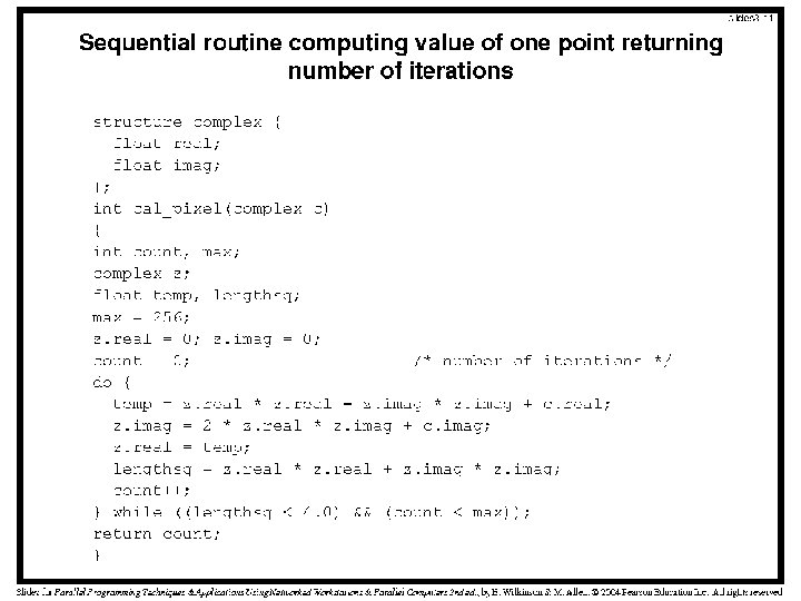
Mandelbrot Set (cont’d) • Including scaling, the code could be of the form: for(x=0; x<disp_width; x++) for(y=0; y<disp_height; y++){ c. real = real_min + ((float)x*scale_real); c. imag = imag_min + ((float)y*scale_imag); color = cal_pixel(c); display(x, y, color); }
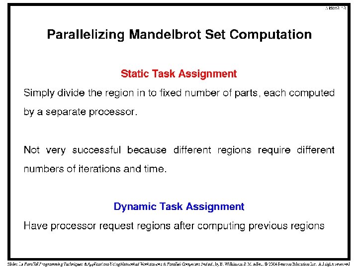

Static Task Assignment • Master for (i = 0, row=0; i < 48; i++, row=row+10) send(&row, P[i]); for (i = 0; i < (480*640); i++) { recv(&c, &color, P[ANY]); display(c, color); }
![Static Task Assignment (cont’d) • Slave (process i) recv(&row, P[MASTER]); for (x = 0;](http://slidetodoc.com/presentation_image_h2/2608f735f28e86314560657198badb3c/image-25.jpg "Static Task Assignment (cont’d) • Slave (process i) recv(&row, P[MASTER]); for (x = 0;")
Static Task Assignment (cont’d) • Slave (process i) recv(&row, P[MASTER]); for (x = 0; i < disp_width; x++) for(y=row; y<row+10; y++){ c. real = real_min + ((float)x*scale_real); c. imag = imag_min + ((float)y*scale_imag); color = cal_pixel(c); send(&c, &color, P[MASTER]); }

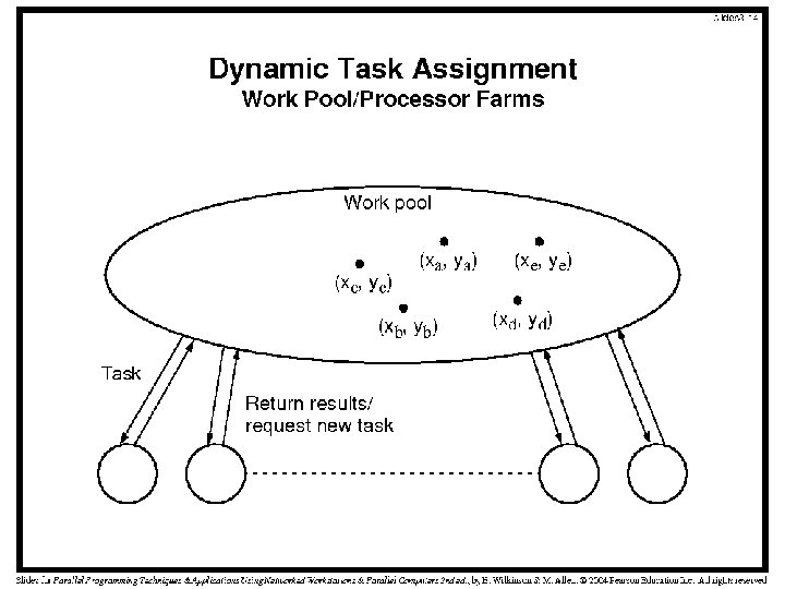
Dynamic Task Assignment • Mandelbrot Set - significant iterative computation per pixel. • The number of iterations will generally be different for each pixel. • Computers may be of different types and speeds in a cluster • Ideally, we want all processors to complete together, achieving a system efficiency of 100%. • Assigning regions of different sizes to different processors also has problems – Need to know a processor’s speed a priori • Work Pool approach (processor farm) – Individual processors are supplied with work when they become idle. • Dynamic load balancing can be achieved using a work-pool approach

Dynamic Task Assignment • Master count=0; /* counter for termination */ row=0; /* row being sent */ for (k = 0, k < num_proc; k++){/*assume num_proc<disp_height*/ send(&row, P[k], data_tag); count++; row++; } do{ recv(&slave, &r, color, P[ANY], result_tag); count--; /* reduce count as rows received */ if(row<display_height){ send(&row, P[SLAVE], data_tag); row++; count++; } else send(&row, P[SLAVE], terminator_tag); display(r, color); } while(count>0);
![Dynamic Task Assignment (cont’d) • Slave recv(&y, P[MASTER], source_tag); while(source_tag==data_tag){ c. imag = imag_min](http://slidetodoc.com/presentation_image_h2/2608f735f28e86314560657198badb3c/image-29.jpg "Dynamic Task Assignment (cont’d) • Slave recv(&y, P[MASTER], source_tag); while(source_tag==data_tag){ c. imag = imag_min")
Dynamic Task Assignment (cont’d) • Slave recv(&y, P[MASTER], source_tag); while(source_tag==data_tag){ c. imag = imag_min + ((float)y*scale_imag); for(x=0; x<disp_width; x++){ c. real = real_min + ((float)x*scale_real); color[x] = cal_pixel(c ); } send(c, color, P[MASTER], result_tag); recv(&y, P[MASTER], source_tage); /* recv next row */ }

Analysis • Exact analysis of the Mandelbrot computation is complicated by not knowing how many iterations are needed for each pixel. • The number of iterations for each pixel is some function of c but cannot exceed max. • Therefore, the sequential time is • • Sequential time complexity of O(n). Let us just consider the static assignment. Three phases: Phase 1: Communication – First, the row number is sent to each slave one data item to each p-1 slaves tcomm 1 = (p-1)(tstartup + tdata)
 • Phase 2: Computation – The slaves perform the Mandelbrot computation in")
Analysis (cont’d) • Phase 2: Computation – The slaves perform the Mandelbrot computation in parallel • Phase 3: Communication – Results are passed back to the master, one row of pixel colors at a time. – Suppose each slave handles u rows and there are v pixels on a row: – For static assignment, u and v will be constant (unless the solution of the image was changed), so we can assume tcomm 2 = k, a constant

Overall Execution Time • Overall, the parallel time is given by where the total number of processors is p
- Slides: 39