Characteristic curves and their responses The method of

Characteristic curves and their responses

The method of Characteristic Curves (Two layer case) Summary of steps • Set 1= a 1 • Construct the ratios a/ 1 for each spacing. • Guess a depth Z ….

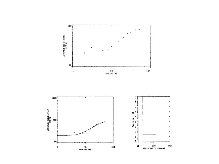
The Inflection Point Depth Estimation Procedure This technique suggests that the depths to various boundaries are related to inflection points in the apparent resistivity measurements. Again, the In-Class data set illustrates the utility of this approach. Apparent resistivities plotted below are shown over the model for both the Schlumberger and Wenner arrays. The inflection points are located, and dropped to the spacing-axis. The technique is suggested too be most applicable for use with the Schlumberger array. A common rule would be that the depth to the top of the high resistivity layer encountered in this survey would be equal to inflection point AB/2 (or l) spacing divided by 2. For the Schlumberger array this would give a depth to the top of the layer of about 12 meters instead of the actual depth of 8. This rule actually works better for the Wenner array. In the case of the Wenner array we would get a depth of about 9 meters. I suggest that a better “rule of thumb” for the Schlumberger array would to divide the inflection point distance by 4 (or even 3) instead of 2.

Resistivity estimation through extrapolation This technique suggests that the actual resistivity of a layer can be estimated by extrapolating the trend of apparent resistivity variations toward some asymptote, as shown in the figure below. The problem with this is being able to correctly guess where the plateau or asymptote actually is. Spacings in the In-Class data set only go out to 50 meters. The model data set (below) used for the inflection point discussion reveals that this asymptote is reached only gradually, in this case at distances of 500 meters and greater. Since most of the layers affecting the apparent resistivity in our surveys will be associated with thin layers, we are unlikely to be able to do this very accurately. The apparent resistivity will vary considerably over that distance rather than rise gradually to resistivities of individual layers. At best the technique offers only a crude estimate.

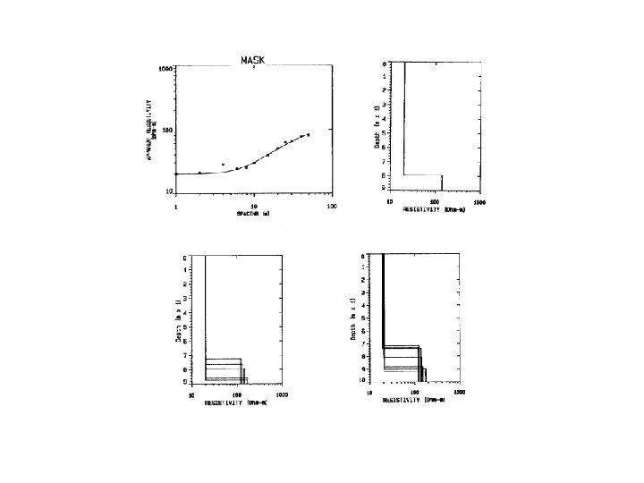
As an alternative to the guess work of convergence on asymptotes and inflection point rules, one can undertake a “characteristic curves” analysis In the graph at right, we have the variations in a/ 1 plotted for three different guesses of Z – the depth to the interface. Plot a/Z ( the Wenner spacing divided by your guess of the depth) versus a/ 1

Each of these curves are associated with a different value of k - the reflection coefficient. The method of Characteristic Curves (Two layer case) Summary of steps ……. • Guess a depth Z • Compute the ratio a/Z • Plot a/ 1 vs. a/Z on the characteristic curves (right) • Select best guess based on the goodness of fit to the characteristic curves. • Determine k (the reflection coefficient) based on the best fit line. • Compute 2, using relationship between k and ‘s

Recall, that once you have determined k, it is straightforward to compute 2 1 = a (shortest a-spacing)

Tri-potential resistivity method 2 a Can you compute the geometrical factors for these various electrode configurations? 3 a -6 a

Increase in apparent resistivity measured by the CCPP electrode array is actually an indicator of a low resistivity – perhaps water filled - fracture zone.

Case History Resistivity Profiling Surveys on the Hopemont Farm in Terra Alta, WV Survey performed by Eb Werner for Dr. Rauch

Survey was conducted for the City of Terra Alta to locate a water well. From Werner and Rauch

The tri-potential resistivity response over an air-filled fracture zone. Model data CPCP CPPC CCPP From Werner and Rauch

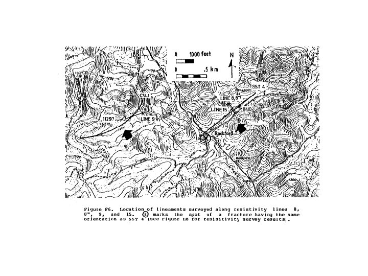
• The Terra Alta surveys conducted by Werner and Rauch employed measurements at three different a-spacings - 10 ft, 20 ft and 40 ft. • Lines were positioned to cross a photolineament and were from 250 to 500 feet in length. • Readings were made at 10 foot intervals. Things to avoid. Conductive materials buried or in contact with the ground. Buried telephone cables and metallic pipelines, fences, metallic posts and overhead power lines

Interpretation approach The apparent resistivity measurements made by Werner and Rauch were interpreted within the context of the tri-potential response predicted by the Carpenter model (see earlier figure). “. . The present problem involves only the confirmation of the existence and exact location of a fracture zone mapped from other information. ” “ … it is only necessary to locate anomalies characteristic of vertical discontinuities …” “ … the graphic plots were inspected visually for those anomaly responses. . ” Anomalous areas were plotted on location maps. “Alignments of such anomalies at or near the location of the postulated fracture zone were accepted as confirmation of the existence of the fracture zone.

Northernmost site - site 1 (see earlier location map) Line 1 is highlighted in red below From Werner and Rauch

N S 10 meter Line 1 20 meter From Werner and Rauch The anomaly around 100 feet is considered to be “data noise” The feature at 320 feet is interpreted to be the “fracture zone” response. Note that this feature is not marked by highs in the CPPC and CPCP measurements The 20 foot a-spacing profile reveals a more pronounced fracture zone anomaly at about 320 feet along the profile. The response suggests high reistivity

Red dots locate prominent “fracture zone” anomalies observed on all three a-spacings Line 1 The blue line indicates the probable location of a major fracture zone. Line 6 Given the 10 foot station spacing location of the zone is accurate to no more than ± 5 feet From Werner and Rauch

N S The fracture zone anomaly appears consistently on Line 6 at approximately 125 feet along the profile 10 Line 6 20 The anomaly broadens as the a -spacing increases because electrodes in the array extend over the anomalous region at greater and greater distances from the array center point. 40 From Werner and Rauch

Northernmost site - site 1 (see earlier location map) Line 1 is highlighted in red below 130 gpm ~400 gpm From Werner and Rauch