CHAPTER VII ANALYSIS OF AREA DATA METU GGIT

CHAPTER VII ANALYSIS OF AREA DATA METU, GGIT 538

7. 1. Introduction In this chapter it is considered to analyze data associated with spatial zones or areas. The areas may be in two different forms: v A regular lattice (pixels in remotely sensed images) v A set of irregular areas (postal or administrative districts) METU, GGIT 538

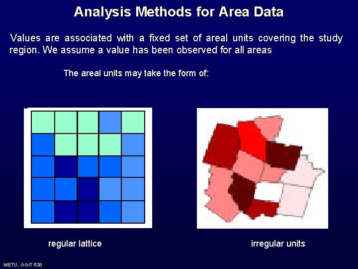
Analysis Methods for Area Data Values are associated with a fixed set of areal units covering the study region. We assume a value has been observed for all areas The areal units may take the form of: regular lattice METU, GGIT 538 irregular units

Analysis Methods for Area Data Basic Objectives: v Not prediction - there are typically no unobserved values, the attribute is exhaustively measured. v Model spatial patterns in the values associated with fixed areas and determine possible explanations for such patterns METU, GGIT 538

The main concern is: ü E. g. Investigating the relationship between disease rates and various socio-economic or environmental factors. METU, GGIT 538

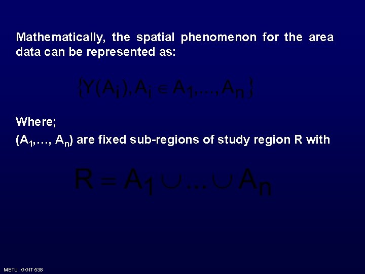
Mathematically, the spatial phenomenon for the area data can be represented as: Where; (A 1, …, An) are fixed sub-regions of study region R with METU, GGIT 538

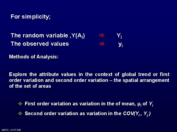
For simplicity; The random variable , Y(Aİ) The observed values Yİ yi Methods of Analysis: Explore the attribute values in the context of global trend or first order variation and second order variation – the spatial arrangement of the set of areas v First order variation as variation in the of mean, μi of Yi v Second order variation as variation in the COV(Yi , Yj ) METU, GGIT 538

7. 2. Case Studies The following data sets will be taken into account when studying the area data: 1. Child mortality in Auckland, New Zealand 2. Socio-economic data for Chinese provinces 3. Census data for enumeration districts in London Borough of Barnet 4. Voting data in 1992 US presidential election 5. Mortality rates and socio-economic measures in English Health Districts 6. Prevalence of human blood group A in Ireland 7. Emissions of nitrogen and ammonia in Europe 8. LANDSAT TM data for part of High Peak region, England METU, GGIT 538

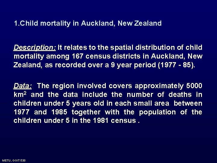
1. Child mortality in Auckland, New Zealand Description: It relates to the spatial distribution of child mortality among 167 census districts in Auckland, New Zealand, as recorded over a 9 year period (1977 - 85). Data: The region involved covers approximately 5000 km 2 and the data include the number of deaths in children under 5 years old in each small area between 1977 and 1985 together with the population of the children under 5 in the 1981 census. METU, GGIT 538

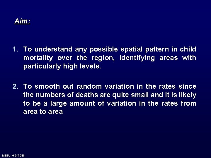
Aim: 1. To understand any possible spatial pattern in child mortality over the region, identifying areas with particularly high levels. 2. To smooth out random variation in the rates since the numbers of deaths are quite small and it is likely to be a large amount of variation in the rates from area to area METU, GGIT 538

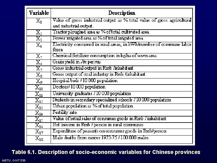
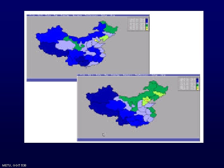
2. Socio-economic data for Chinese provinces Description: It concerns the socio-economic measures of civil divisions in China. Within the People’s Republic of China inequalities between different regions should not, in theory, exist. Since mid-1970’s the push towards higher levels of economic growth has meant that historical inequalities have persisted and been acknowledged as inevitable. Industrialization had led to concentrations of better paid and more educated in urban areas and poorer population in more rural areas. METU, GGIT 538

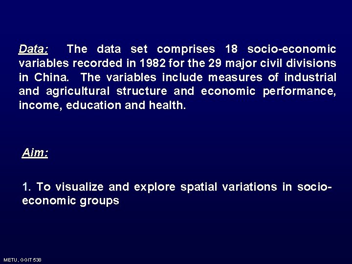
Data: The data set comprises 18 socio-economic variables recorded in 1982 for the 29 major civil divisions in China. The variables include measures of industrial and agricultural structure and economic performance, income, education and health. Aim: 1. To visualize and explore spatial variations in socioeconomic groups METU, GGIT 538

Table 6. 1. Description of socio-economic variables for Chinese provinces METU, GGIT 538

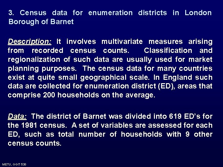
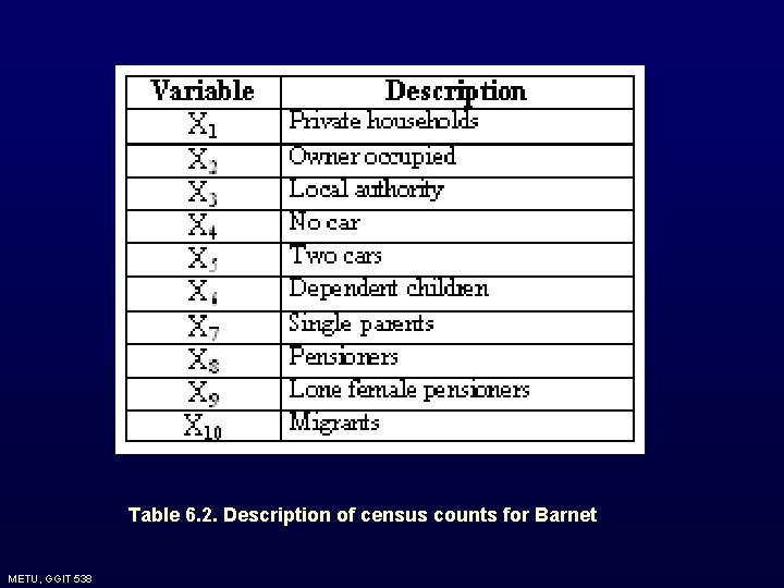
3. Census data for enumeration districts in London Borough of Barnet Description: It involves multivariate measures arising from recorded census counts. Classification and regionalization of such data are usually used for market planning purposes. The census data for many countries exist at quite small geographical scale. In England such data are collected for enumeration district (ED), areas that comprise 200 households on the average. Data: The district of Barnet was divided into 619 ED’s for the 1981 census. A set of variables are assessed for each ED, such as total number of households with 9 other census counts. METU, GGIT 538

Table 6. 2. Description of census counts for Barnet METU, GGIT 538

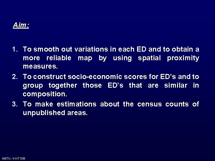
Aim: 1. To smooth out variations in each ED and to obtain a more reliable map by using spatial proximity measures. 2. To construct socio-economic scores for ED’s and to group together those ED’s that are similar in composition. 3. To make estimations about the census counts of unpublished areas. METU, GGIT 538

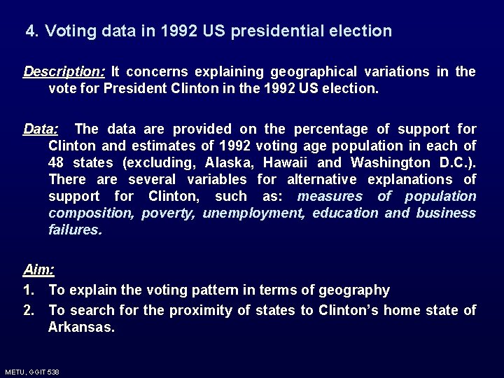
4. Voting data in 1992 US presidential election Description: It concerns explaining geographical variations in the vote for President Clinton in the 1992 US election. Data: The data are provided on the percentage of support for Clinton and estimates of 1992 voting age population in each of 48 states (excluding, Alaska, Hawaii and Washington D. C. ). There are several variables for alternative explanations of support for Clinton, such as: measures of population composition, poverty, unemployment, education and business failures. Aim: 1. To explain the voting pattern in terms of geography 2. To search for the proximity of states to Clinton’s home state of Arkansas. METU, GGIT 538

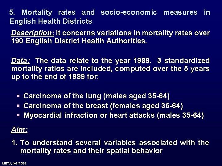
5. Mortality rates and socio-economic measures in English Health Districts Description: It concerns variations in mortality rates over 190 English District Health Authorities. Data: The data relate to the year 1989. 3 standardized mortality ratios are included, computed over the 5 years up to the end of 1989 for: § Carcinoma of the lung (males aged 35 -64) § Carcinoma of the breast (females aged 35 -64) § Myocardial infraction or heart attacks (males 35 -64) Aim: 1. To understand several variables associated with the mortality rates and their spatial behavior METU, GGIT 538

6. Prevalence of human blood group A in Ireland Description: It concerns distribution of adult population in Eire that has blood group A. Data: The proportion of adults with blood group A was measured in 1958 in samples drawn from the population of each of the 26 Irish counties (totally 55 000 samples) Aim: • • • To describe the spatial variations in the proportions over the set of counties. To search for if the variation in blood group can be explained by settlement history. To investigate if the extent of simple variables are sufficient enough to explain the variation in blood group. METU, GGIT 538

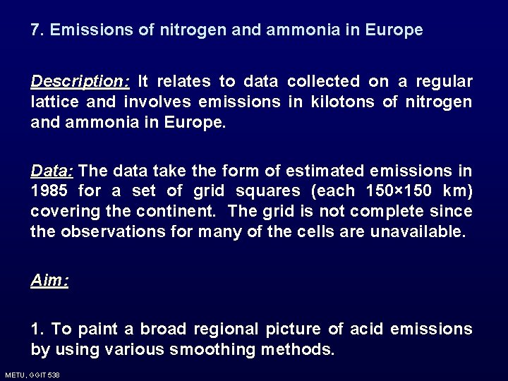
7. Emissions of nitrogen and ammonia in Europe Description: It relates to data collected on a regular lattice and involves emissions in kilotons of nitrogen and ammonia in Europe. Data: The data take the form of estimated emissions in 1985 for a set of grid squares (each 150× 150 km) covering the continent. The grid is not complete since the observations for many of the cells are unavailable. Aim: 1. To paint a broad regional picture of acid emissions by using various smoothing methods. METU, GGIT 538

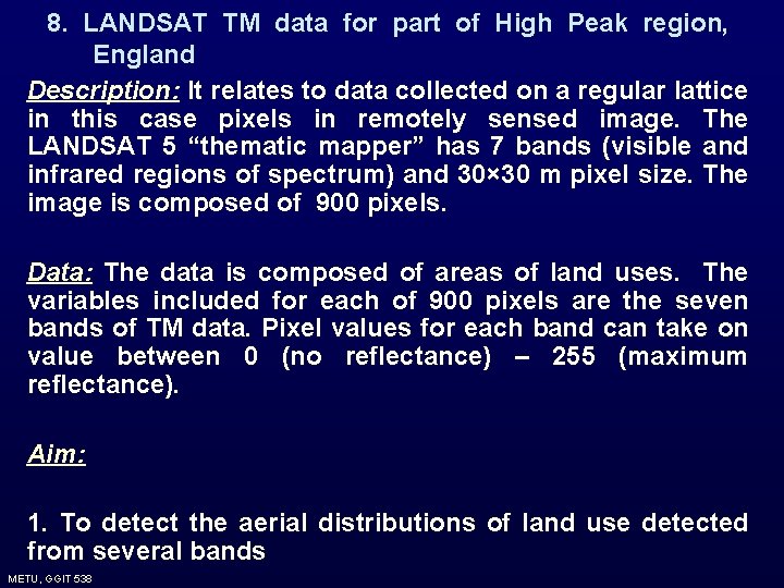
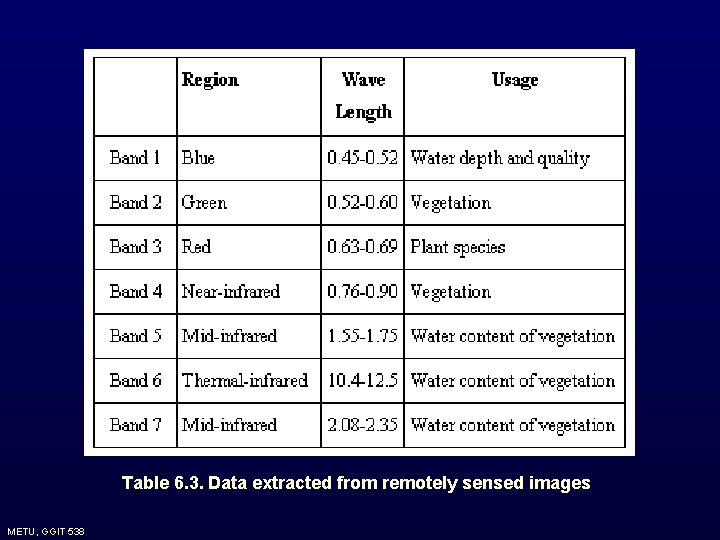
8. LANDSAT TM data for part of High Peak region, England Description: It relates to data collected on a regular lattice in this case pixels in remotely sensed image. The LANDSAT 5 “thematic mapper” has 7 bands (visible and infrared regions of spectrum) and 30× 30 m pixel size. The image is composed of 900 pixels. Data: The data is composed of areas of land uses. The variables included for each of 900 pixels are the seven bands of TM data. Pixel values for each band can take on value between 0 (no reflectance) – 255 (maximum reflectance). Aim: 1. To detect the aerial distributions of land use detected from several bands METU, GGIT 538

Table 6. 3. Data extracted from remotely sensed images METU, GGIT 538

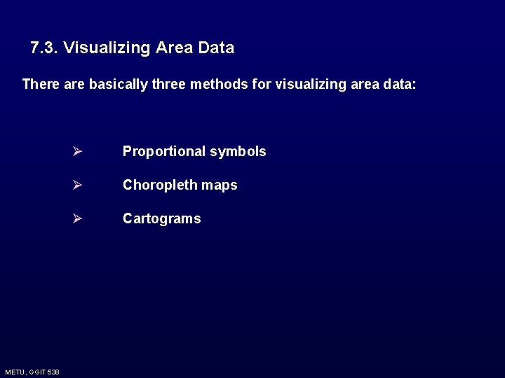
7. 3. Visualizing Area Data There are basically three methods for visualizing area data: METU, GGIT 538 Ø Proportional symbols Ø Choropleth maps Ø Cartograms

7. 3. Visualizing Area Data Proportional symbols : They are superimposed over the areal units Symbols are proportionate to the attribute value of the area METU, GGIT 538

Coropleth Maps: The coropleth map is a map where each of the areas Ai is colored or shaded according to a discrete scale based on the value of the attribute of interest within that area. Therefore; v Attribute of interest is scaled to a set of discrete ranges or classes v Each zone is shaded or colored according to its attribute value The number of classes and the corresponding class intervals can be based on several different criteria. METU, GGIT 538

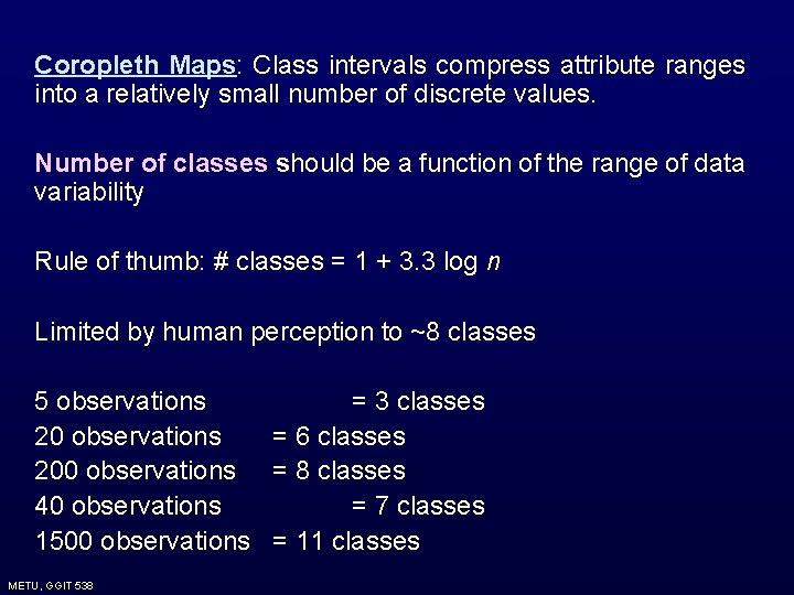
Coropleth Maps: Class intervals compress attribute ranges into a relatively small number of discrete values. Number of classes should be a function of the range of data variability Rule of thumb: # classes = 1 + 3. 3 log n Limited by human perception to ~8 classes 5 observations = 3 classes 20 observations = 6 classes 200 observations = 8 classes 40 observations = 7 classes 1500 observations = 11 classes METU, GGIT 538

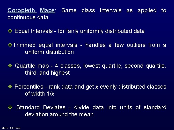
Coropleth Maps: Same class intervals as applied to continuous data v Equal Intervals - for fairly uniformly distributed data v. Trimmed equal intervals - handles a few outliers from a uniform distribution v Quartile map - 4 classes, lowest quartile, second quartile, third, and highest v Percentiles - rank data and get x evenly distributed classes of width 1/x v Standard Deviates - divide data into units of standard deviation around the mean METU, GGIT 538

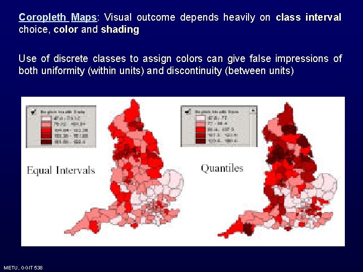
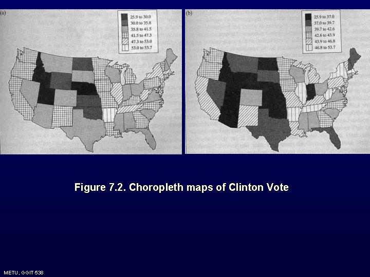
Coropleth Maps: Visual outcome depends heavily on class interval choice, color and shading Use of discrete classes to assign colors can give false impressions of both uniformity (within units) and discontinuity (between units) METU, GGIT 538

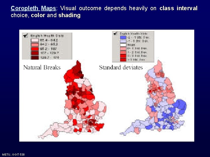
Coropleth Maps: Visual outcome depends heavily on class interval choice, color and shading METU, GGIT 538

Figure 7. 2. Choropleth maps of Clinton Vote METU, GGIT 538

Problems of Coropleth Mapping 1. They may be very misleading. When the class intervals are changed different interpretations can be achieved. 2. Physically large areas tend to dominate to display, in a way which may be quite in appropriate for the type of data being mapped. E. g. In mapping socio-economic data, large and sparsely populated rural areas may dominate because of the visual intrusiveness of the large aerial units. METU, GGIT 538

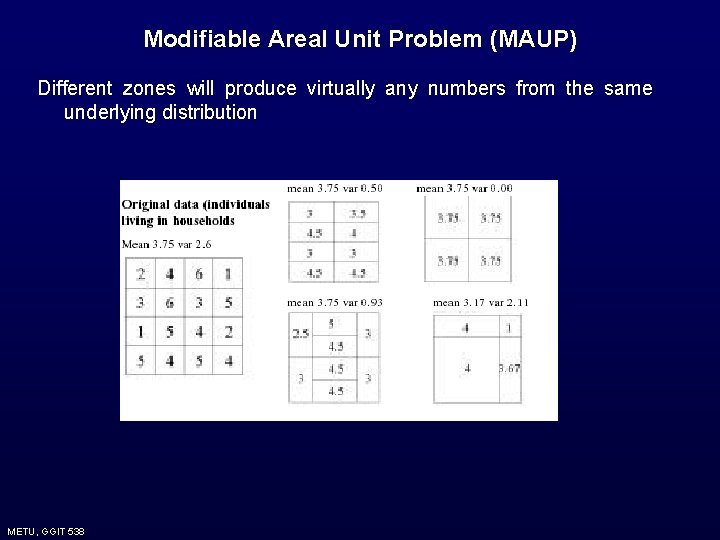
3. When the attribute of interest has arisen from aggregate of individual data to the areas, it must be appreciated that these areas may have been designed rather arbitrarily on the basis of administrative or enumeration purposes. Hence any pattern that is observed may be as much a function of the zone boundaries chosen (modifiable aerial unit problem) METU, GGIT 538

Modifiable Areal Unit Problem (MAUP) Different zones will produce virtually any numbers from the same underlying distribution METU, GGIT 538

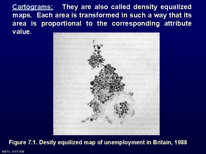
Cartograms: They are also called density equalized maps. Each area is transformed in such a way that its area is proportional to the corresponding attribute value. Figure 7. 1. Desity equilized map of unemployment in Britain, 1988 METU, GGIT 538

7. 4. Exploring Area Data Exploration of the area data addresses first and second order effects. Whatever the method, the main problem is to determine the proximity measures of the observations when they relate to irregularly shaped aerial units. METU, GGIT 538

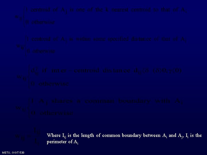
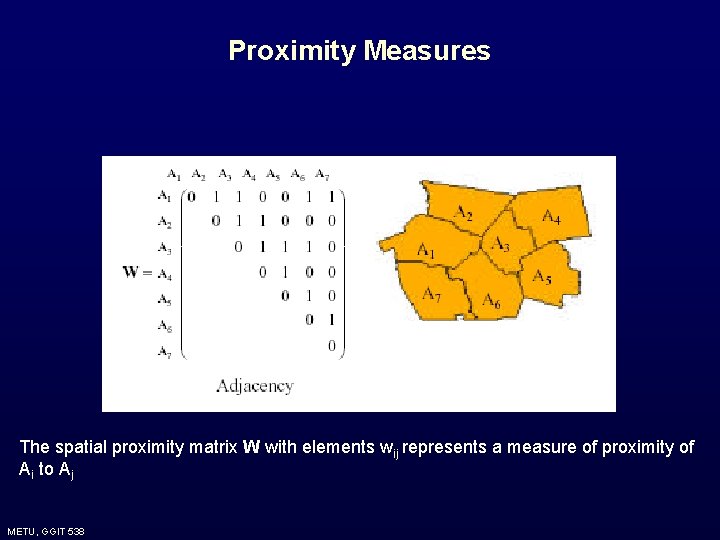
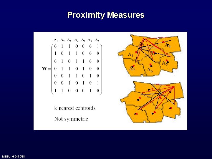
7. 4. 1. Proximity Measures For the area data how to define spatial proximity measures between each of the areas Ai, is the basic issue. The crudest way is to use the centroids of the areas. However, doing so leads to disregard some aspects of the spatial nature of these areas. Hence it is needed to use more general proximity measures. The general tool is the use of idea of (n×n) spatial proximity matrix W, whose elements (wij) represents a measure of the spatial proximity of areas Ai and Aj. The choice of wij depends on the sort of data. The possible wij are: METU, GGIT 538

Where Iij is the length of common boundary between Ai and Aj, Ii is the perimeter of Ai METU, GGIT 538

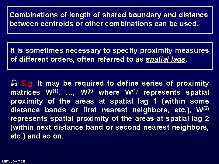
Combinations of length of shared boundary and distance between centroids or other combinations can be used. It is sometimes necessary to specify proximity measures of different orders, often referred to as spatial lags. E. g. It may be required to define series of proximity matrices W(1), …, W(k) where W(1) represents spatial proximity of the areas at spatial lag 1 (within some distance bands or first nearest neighbors, etc. ), W(2) represents spatial proximity of the areas at spatial lag 2 (within next distance band or second nearest neighbors, etc. ) and so on. METU, GGIT 538

Proximity Measures The spatial proximity matrix W with elements wij represents a measure of proximity of Ai to Aj METU, GGIT 538

Proximity Measures METU, GGIT 538

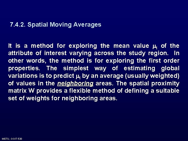
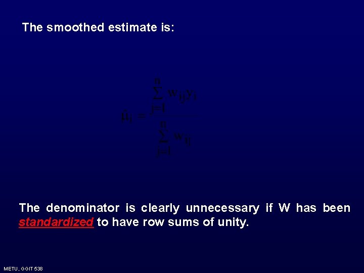
7. 4. 2. Spatial Moving Averages It is a method for exploring the mean value i of the attribute of interest varying across the study region. In other words, the method is for exploring the first order properties. The simplest way of estimating global variations is to predict i by an average (usually weighted) of values in the neighboring areas. The spatial proximity matrix W provides a flexible method of defining a suitable set of weights for neighboring areas. METU, GGIT 538

The smoothed estimate is: The denominator is clearly unnecessary if W has been standardized to have row sums of unity. METU, GGIT 538

METU, GGIT 538

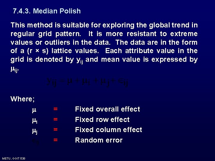
7. 4. 3. Median Polish This method is suitable for exploring the global trend in regular grid pattern. It is more resistant to extreme values or outliers in the data. The data are in the form of a (r × s) lattice values. Each attribute value in the grid is denoted by yij and mean value is expressed by ij. Where; i j METU, GGIT 538 = = Fixed overall effect Fixed row effect Fixed column effect Random error

Then a model can be fitted by an ordinary analysis of variance, where the estimates of , i, j would be based on row and column means. Median polish on the other hand estimates the effects using medians rather than means. Hence it is more robust to extreme values. METU, GGIT 538

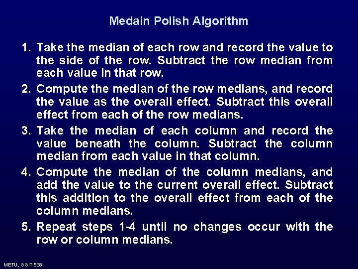
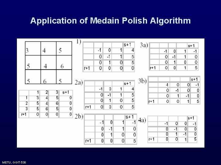
Medain Polish Algorithm 1. Take the median of each row and record the value to the side of the row. Subtract the row median from each value in that row. 2. Compute the median of the row medians, and record the value as the overall effect. Subtract this overall effect from each of the row medians. 3. Take the median of each column and record the value beneath the column. Subtract the column median from each value in that column. 4. Compute the median of the column medians, and add the value to the current overall effect. Subtract this addition to the overall effect from each of the column medians. 5. Repeat steps 1 -4 until no changes occur with the row or column medians. METU, GGIT 538

Application of Medain Polish Algorithm METU, GGIT 538

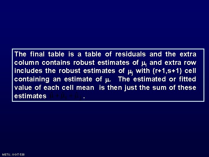
The final table is a table of residuals and the extra column contains robust estimates of i and extra row includes the robust estimates of j with (r+1, s+1) cell containing an estimate of . The estimated or fitted value of each cell mean is then just the sum of these estimates. METU, GGIT 538

Problems of Median Polish 1. It attempts to decompose trend according to the directions of the grid which often has no relationship to the spatial orientation of the trend. If the trends are essentially circular, this does not create too much problem. However, if it is elongated in a direction it creates problems. 2. One is unable in any way to control the degree of smoothing applied. METU, GGIT 538

Median polish can be adopted for systems of aerial units other than regular lattices, by assigning each area to the closest cell of some suitably chosen grid overlaid on the areas. These grids can not be equally spaced in either direction. In some cases two areas can be assigned to one gird and some grids may contain no area. Median polish does not affected by these situations. METU, GGIT 538

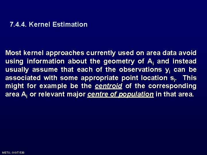
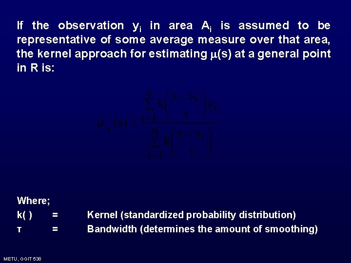
7. 4. 4. Kernel Estimation Most kernel approaches currently used on area data avoid using information about the geometry of Ai and instead usually assume that each of the observations yi can be associated with some appropriate point location si. This might for example be the centroid of the corresponding area Ai or relevant major centre of population in that area. METU, GGIT 538

If the observation yi in area Ai is assumed to be representative of some average measure over that area, the kernel approach for estimating (s) at a general point in R is: Where; k( ) = τ = METU, GGIT 538 Kernel (standardized probability distribution) Bandwidth (determines the amount of smoothing)

When observations yi in areas Ai represent totals such as census counts then the above approach is not applicable. An average value at s of such a count is meaningless concept and it is needed to think in terms of an estimate of density at s say λ(s). An obvious estimate is: METU, GGIT 538

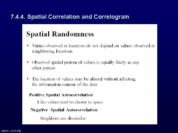
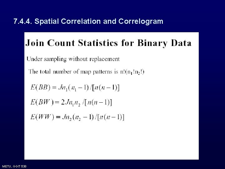
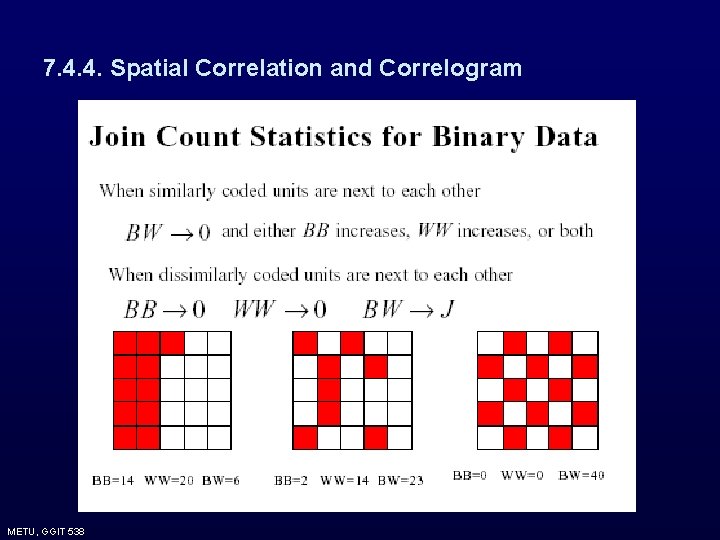
7. 4. 4. Spatial Correlation and Correlogram The methods discussed up to now deal with exploring the first order characteristics of the data or estimating the mean or expected value of the process varying over the study region. Spatial correlation and correlogram concern with exploration of the spatial dependence of deviations in attribute values from their mean, i. e. second order properties. In area data, estimates of spatial autocorrelation rather than covariance are typically used Autocorrelation v Correlation of a random variable with itself v In time domain: correlation between value at time t and at time t - h v In spatial domain: correlation between value at a location i and neighboring locations j METU, GGIT 538

7. 4. 4. Spatial Correlation and Correlogram METU, GGIT 538

7. 4. 4. Spatial Correlation and Correlogram METU, GGIT 538

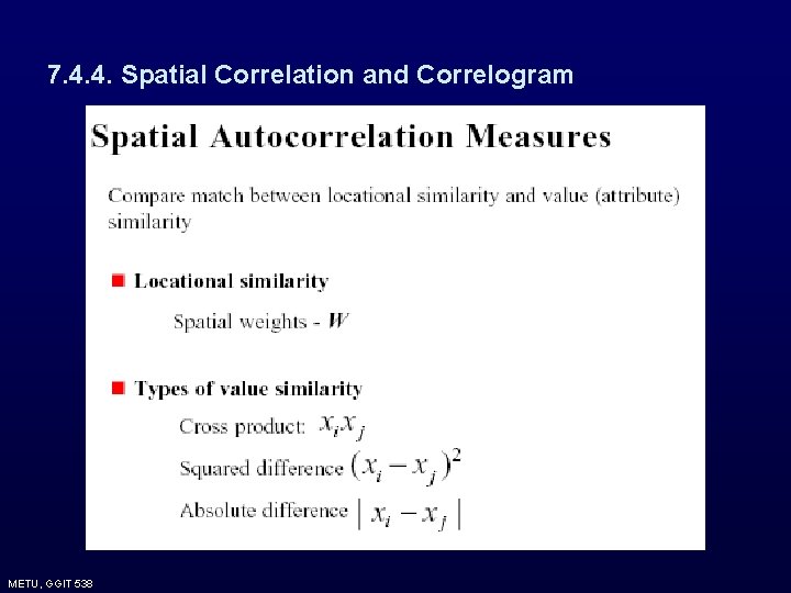
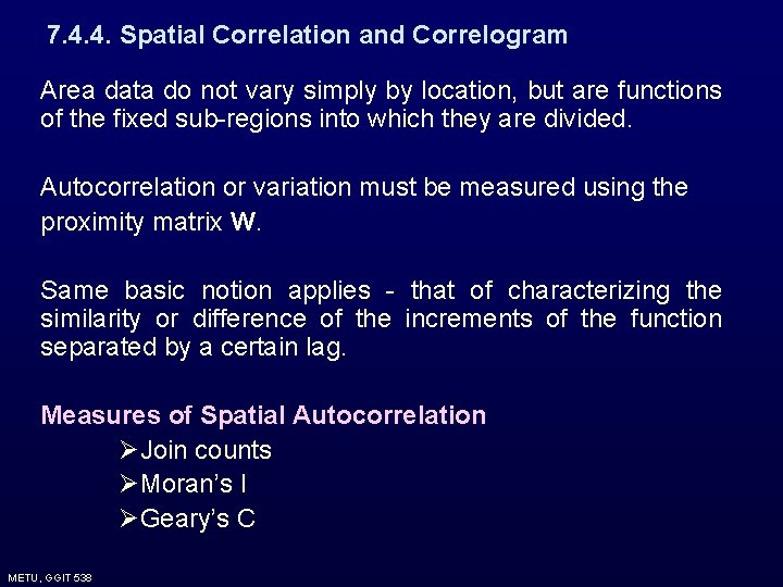
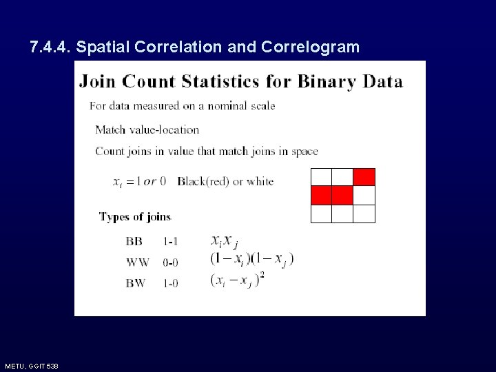
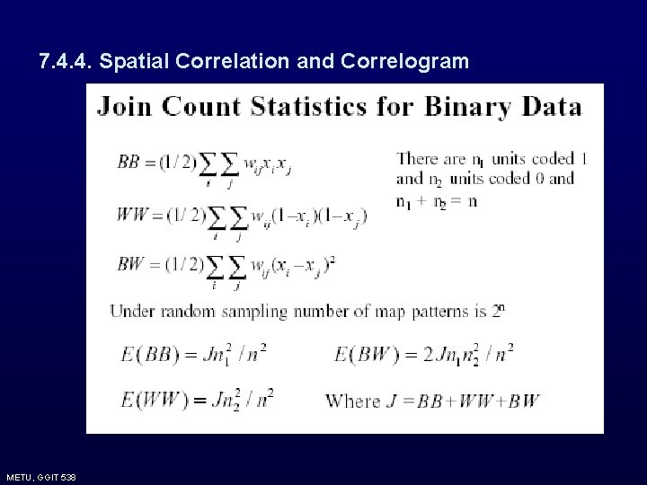
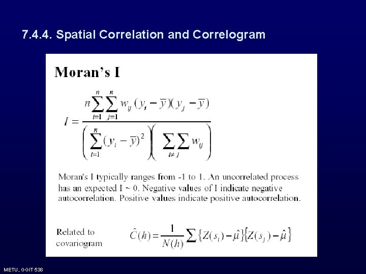
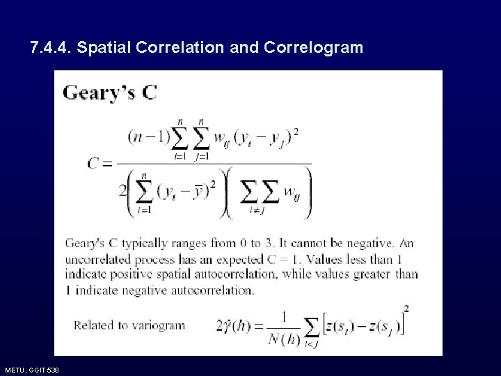
7. 4. 4. Spatial Correlation and Correlogram Area data do not vary simply by location, but are functions of the fixed sub-regions into which they are divided. Autocorrelation or variation must be measured using the proximity matrix W. Same basic notion applies - that of characterizing the similarity or difference of the increments of the function separated by a certain lag. Measures of Spatial Autocorrelation ØJoin counts ØMoran’s I ØGeary’s C METU, GGIT 538

7. 4. 4. Spatial Correlation and Correlogram METU, GGIT 538

7. 4. 4. Spatial Correlation and Correlogram METU, GGIT 538

7. 4. 4. Spatial Correlation and Correlogram METU, GGIT 538

7. 4. 4. Spatial Correlation and Correlogram METU, GGIT 538

7. 4. 4. Spatial Correlation and Correlogram METU, GGIT 538

7. 4. 4. Spatial Correlation and Correlogram METU, GGIT 538

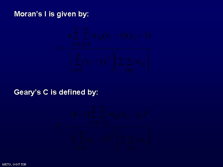
Moran’s I is given by: Geary’s C is defined by: METU, GGIT 538

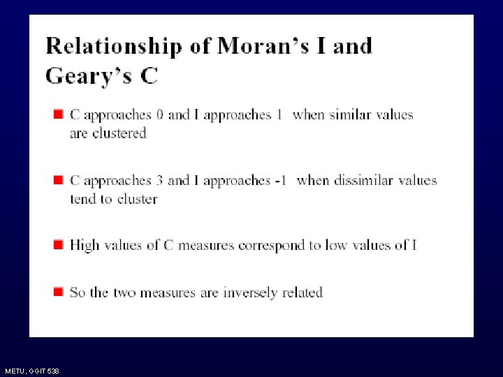
None of I and C statistics are constrained to lie within ( -1, 1). However, they can be adjusted by their theoretical bounds to force to lie between (-1, 1). The theoretical bound for I is: Hence if I is divided by this bound it would be restricted to lie between (-1, 1). METU, GGIT 538

METU, GGIT 538

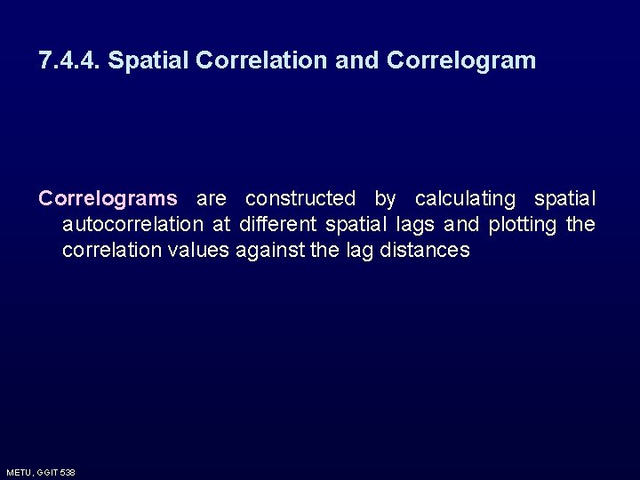
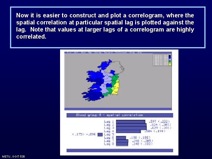
7. 4. 4. Spatial Correlation and Correlograms are constructed by calculating spatial autocorrelation at different spatial lags and plotting the correlation values against the lag distances METU, GGIT 538

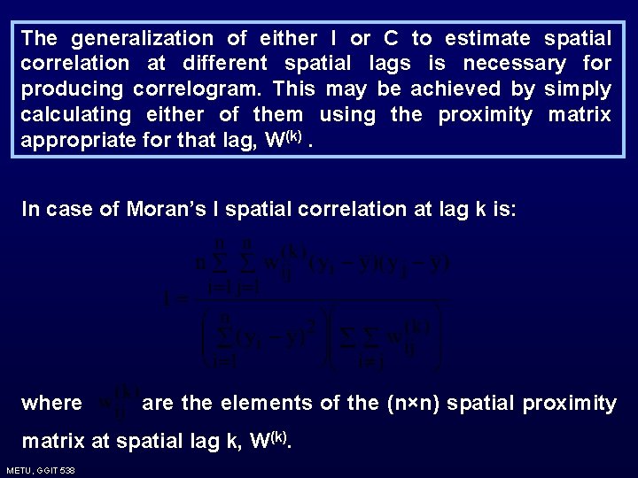
The generalization of either I or C to estimate spatial correlation at different spatial lags is necessary for producing correlogram. This may be achieved by simply calculating either of them using the proximity matrix appropriate for that lag, W(k). In case of Moran’s I spatial correlation at lag k is: where are the elements of the (n×n) spatial proximity matrix at spatial lag k, W(k). METU, GGIT 538

Now it is easier to construct and plot a correlogram, where the spatial correlation at particular spatial lag is plotted against the lag. Note that values at larger lags of a correlogram are highly correlated. METU, GGIT 538

7. 5. Modeling Area Data • Non-spatial regression models • Spatial regression models • Tests for spatial correlations METU, GGIT 538

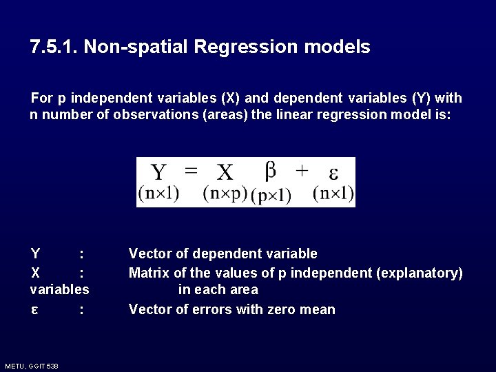
7. 5. 1. Non-spatial Regression models For p independent variables (X) and dependent variables (Y) with n number of observations (areas) the linear regression model is: Y : X : variables ε : METU, GGIT 538 Vector of dependent variable Matrix of the values of p independent (explanatory) in each area Vector of errors with zero mean

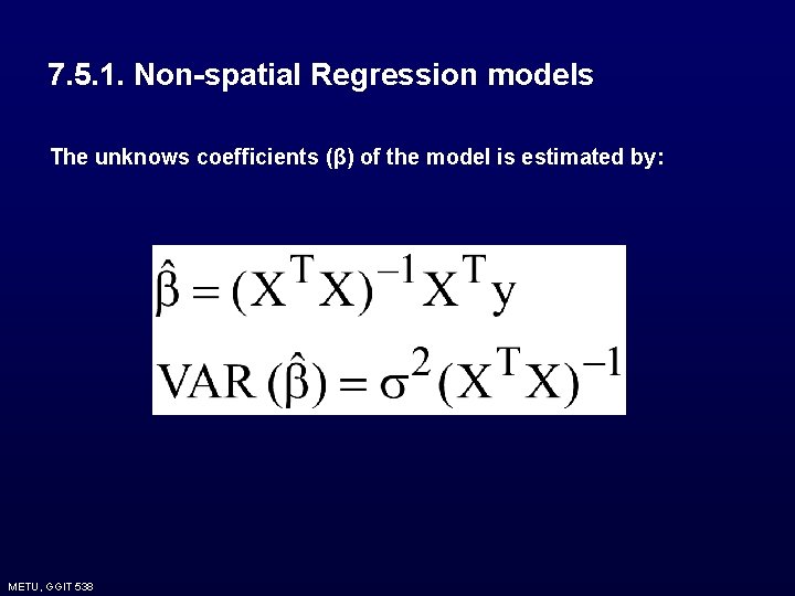
7. 5. 1. Non-spatial Regression models The unknows coefficients (β) of the model is estimated by: METU, GGIT 538

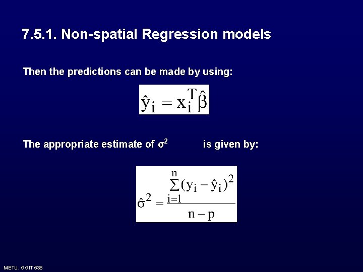
7. 5. 1. Non-spatial Regression models Then the predictions can be made by using: The appropriate estimate of σ2 METU, GGIT 538 is given by:

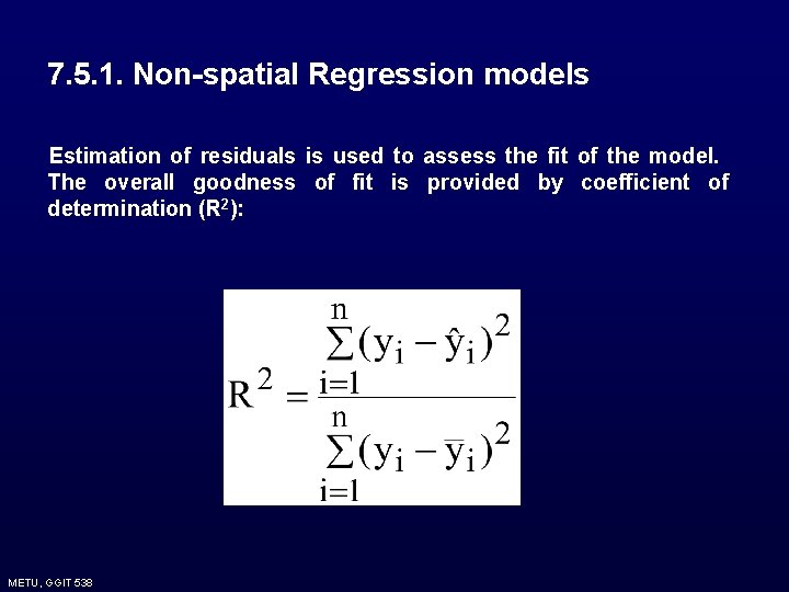
7. 5. 1. Non-spatial Regression models Estimation of residuals is used to assess the fit of the model. The overall goodness of fit is provided by coefficient of determination (R 2): METU, GGIT 538

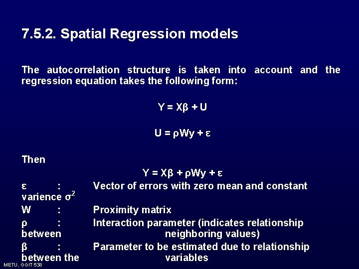
7. 5. 2. Spatial Regression models The autocorrelation structure is taken into account and the regression equation takes the following form: Y = Xβ + U U = ρWy + ε Then ε : varience σ2 W : ρ : between β : between the METU, GGIT 538 Y = Xβ + ρWy + ε Vector of errors with zero mean and constant Proximity matrix Interaction parameter (indicates relationship neighboring values) Parameter to be estimated due to relationship variables

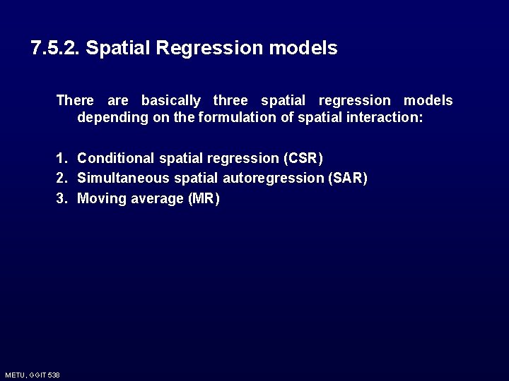
7. 5. 2. Spatial Regression models There are basically three spatial regression models depending on the formulation of spatial interaction: 1. Conditional spatial regression (CSR) 2. Simultaneous spatial autoregression (SAR) 3. Moving average (MR) METU, GGIT 538

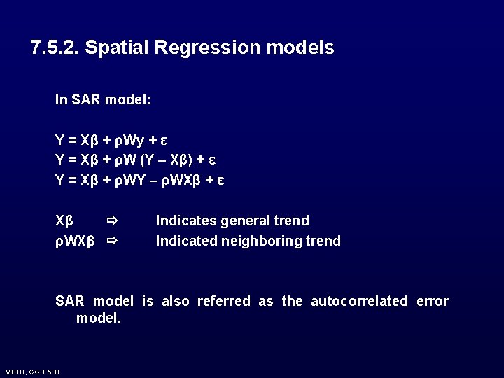
7. 5. 2. Spatial Regression models In SAR model: Y = Xβ + ρWy + ε Y = Xβ + ρW (Y – Xβ) + ε Y = Xβ + ρWY – ρWXβ + ε Xβ ρWXβ Indicates general trend Indicated neighboring trend SAR model is also referred as the autocorrelated error model. METU, GGIT 538

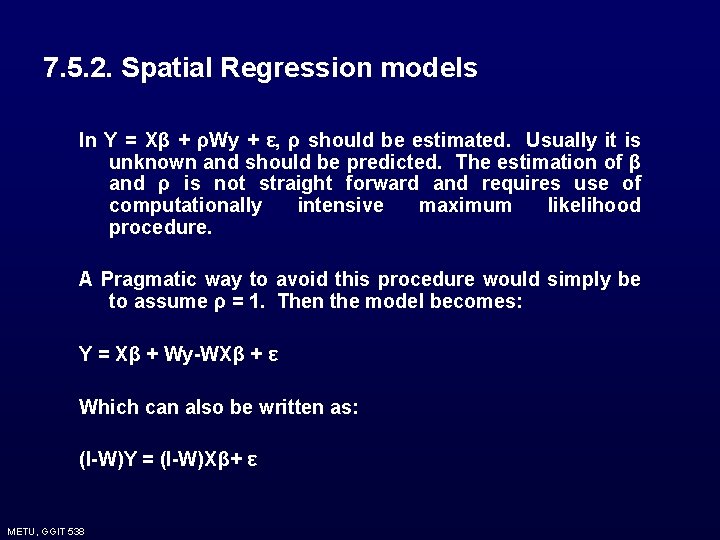
7. 5. 2. Spatial Regression models In Y = Xβ + ρWy + ε, ρ should be estimated. Usually it is unknown and should be predicted. The estimation of β and ρ is not straight forward and requires use of computationally intensive maximum likelihood procedure. A Pragmatic way to avoid this procedure would simply be to assume ρ = 1. Then the model becomes: Y = Xβ + Wy-WXβ + ε Which can also be written as: (I-W)Y = (I-W)Xβ+ ε METU, GGIT 538

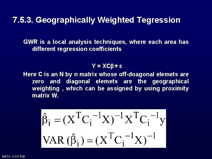
7. 5. 3. Geographically Weighted Tegression GWR is a local analysis techniques, where each area has different regression coefficients Y = XCβ+ ε Here C is an N by n matrix whose off-doagonal elemets are zero and diagonal elemets are the geographical weighting , which can be assigned by using proximity matrix W. METU, GGIT 538