Chapter Two Reliability Function Topics Unreliability Function Reliability

Chapter Two Reliability Function Topics: • Unreliability Function • Reliability Function Derivation Process ü Exponential Distribution ü Weibull Distribution ü Normal Distribution

Unreliability Function • The reliability function can be derived using the definition of the cumulative density function. • Note that the probability of an event happening by time t based on a continuous distribution given by f(x), (or f(t) since our random variable of interest in life data analysis is time) is given by: • One could also equate this event to the probability of a unit failing by time t, since the event of interest in life data analysis is the failure of an item.

• This defines the unreliability function, Q(t), which is the probability of failure, or the probability that the time-to-failure is in the region of 0 (or γ) and t. • So, from the previous equation, we have:

Reliability Function • In this situation, there are only two mutually exclusive situations that can occur: success or failure. • Since reliability and unreliability are the probabilities of two mutually exclusive states, the sum of these probabilities is always equal to unity. So then: Where R(t) is the reliability function

• Conversely, the pdf can be defined in terms of the reliability function as:

Relationship between the Reliability Function & CDF • The following figure illustrates the relationship between the reliability function and the cdf, or the unreliability function.

Reliability Function Derivation Process • We will illustrate the reliability function derivation process with the exponential distribution. • The exponential distribution, the most basic and widely used reliability prediction formula, models machines with the constant failure rate, or the flat section of the bathtub curve. • Most industrial machines spend most of their lives in the constant failure rate, so it is widely applicable.

• The pdf of the exponential distribution is given by: λ = Failure rate (1/MTBF, or 1/MTTF) t = operating time, life, or age, in hours, cycles, miles, actuations, etc. e = base of the natural logarithms (2. 71828) • The exponential PDF represents a random occurrence over time • Hence, the reliability function for the exponential distribution is:

• As λ is decreased, the distribution is stretched out to the right, • As λ is increased, the distribution is pushed toward the origin. • This distribution has no shape parameter as it has only one shape, (i. e. , the exponential, and the only parameter it has is the failure rate, λ ). • The location parameter, ϒ, is zero.

• The distribution starts at t = 0 at the level of f(t = 0) = λ and decreases thereafter exponentially and monotonically as t increases, and is convex. • As , t approaches infinity, f(t) approaches zero. • The pdf can be thought of as a special case of the Weibull pdf withϒ = 0 and β = 1 and.

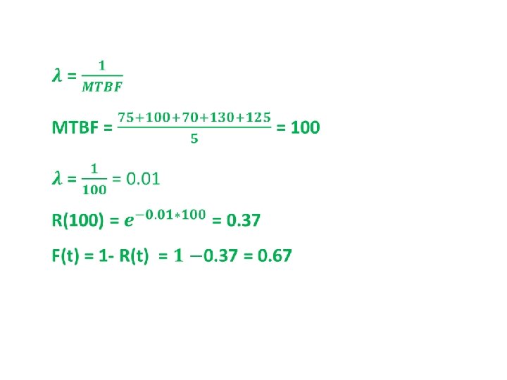
Example •

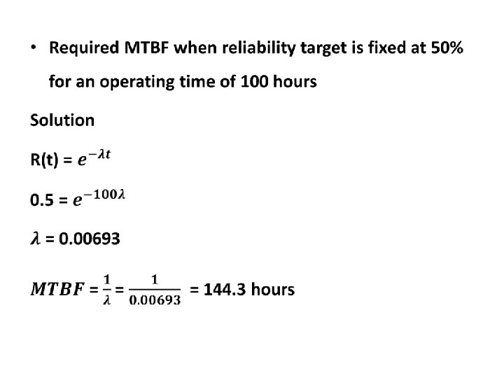
• Operating optimum time when reliability target is 50%

The 2 -Parameter Exponential Distribution • The 2 -parameter exponential pdf is given by: • Where ϒ is the location parameter. • The location parameter, ϒ , if positive, shifts the beginning of the distribution by a distance of to the right of the origin, signifying that the chance failures start to occur only after hours of operation, and cannot occur before • The scale parameter is • The exponential pdf has no shape parameter, as it has only one shape. • The distribution starts at t=ϒ at the level of f(t=ϒ ) = λ and decreases thereafter exponentially and monotonically as t increases beyond ϒ and is convex. • As , t approaches infinity, f(t) approaches zero.

The Mean or MTTF The mean, or mean time to failure (MTTF) is given by: • Note that when ϒ = 0, the MTTF is the inverse of the exponential distribution's constant failure rate. • This is only true for the exponential distribution. • Most other distributions do not have a constant failure rate. • Consequently, the inverse relationship between failure rate and MTTF does not hold for these other distributions

• Different other distributions exist, such as the Weibull, normal, etc. , and each one of them has a predefined f(t). • These distributions were formulated by statisticians, mathematicians and/or engineers to mathematically model or represent certain behavior. • For example, the Weibull distribution was formulated by Walloddi Weibull and thus it bears his name. • Some distributions tend to better represent life data and are most commonly referred to as lifetime distributions.

• However, the exponential distribution and the Weibull distribution are the two most widely applied distributions to reliability engineering.

• For the derivation of the reliability functions for other distributions, including the Weibull, normal and lognormal, see Relia. Soft's Life Data Analysis Online at http: //reliawiki. org/index. php/Life_Data_Analysis _Reference_Book.