Chapter Two Conversion Reactor Sizing 2 1 Definition

Chapter Two: Conversion & Reactor Sizing 2. 1 Definition of Conversion Choose one of reactants (usually limiting reactant) as basis of calculation & then relate other species involved in reaction to this basis.

Develop stoichiometric relationships & design equations by considering general reaction: Uppercase letters represent chemical species & Lowercase letters = stoichiometric coefficients

Taking species A as our basis of calculation, & dividing reaction expression through by stoichiometric coefficient of species A:

To answer "How can we quantify how far a reaction [e. g. , Equation (2 -2)] proceeds to the right? " or "How many moles of C are formed for every mole A consumed? “ these questions is to define a parameter called conversion. Conversion XA is number of moles of A reacted per mole of A fed to system:

For irreversible Xmax=1. 0, i. e. , conversion. reactions, complete For reversible reactions, maximum conversion is equilibrium conversion Xe (i. e. , Xmax = Xe).

2. 2 Batch Reactor Design Equations In most batch reactors, the longer a reactant stays in the reactor, the more the reactant is converted to product until either equilibrium is reached or reactant is exhausted.

Consequently, in batch systems, X is a function of time reactants spend in reactor. If NA 0 is number of moles of A initially in reactor, then total number of moles of A that have reacted after a time t is [NA 0 X]

Now, NA that remain in reactor after a time t, can be expressed in terms of NA 0 & X: When no spatial variations in reaction rate exist, mole balance on species A for a batch system is given by following eq. [Eq. (1 -5)]:

In Eq. (2 -2), reactant A is disappearing; therefore, we multiply both sides of Eq. (2 -5) by -1 to obtain mole balance for batch reactor in form: Rate of disappearance of A, -r. A, in this reaction might be given by a rate law similar to Eq. (1 -2), such as -r. A = k CACB

For batch reactors, we are interested in determining how long to leave reactants in reactor to achieve a certain X.

To determine this time, write mole balance, Eq. (2 -5), in terms of X by differentiating Eq. (2 -4) with respect to time, remembering that NA 0 is number of moles of A initially present constant with respect to time. Combining above with Eq. (2 -5) yields (2 -6)

Eq. (2 -6) differential form of design equation for a batch reactor in terms of X. For a constant-volume batch reactor, V = V 0, Eq. (2 -5) can be arranged into form Eq. (2 -7), used for analyzing rate data in a batch reactor

To determine time to achieve a specified X, separate variables in Eq. (2 -6): Integrating with limits that reaction begins at (i. e. , t = 0, X = 0), to obtain time t necessary to achieve a X in a batch reactor Eq. (2 -9) is integral form of equation for a batch reactor. design

2. 3 Design Equations for Flow Reactors For Continuous-flow systems, time usually increases with increasing reactor volume. e. g. , the bigger/longer the reactor, the more time it will take reactants to flow completely through reactor & thus, more time to react.

Consequently, X is a function of reactor volume V. If FA 0 fed to a system operated at steady state, molar rate at which species A is reacting within entire system will be FA 0 X.

Rearranging gives For liquid systems, CA 0 is commonly given in terms of molarity, for example,

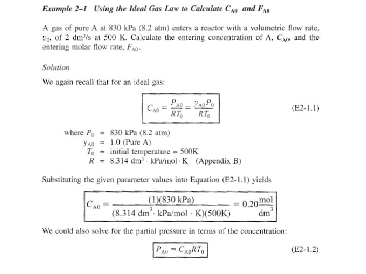
For gas systems, CA 0 can be calculated from entering T & P using ideal gas law or some other gas law. For an ideal gas:

Size of reactor will depend on flow rate, reaction kinetics, reactor conditions, & desired conversion. Let's first calculate entering molar flow rate.

However, since pure A enters, total pressure & partial pressure entering are same. Entering molar flow rate, FA 0, is just product of entering, CA 0, & entering, ν 0:

Use (FA 0= 0. 4 mol/s) together with either Table 2 -2 or Fig. 2 -1 to size & evaluate a number of reactor schemes in Examples 2 -2 through 2 -5.

Relationship [Eq. (2 -10)] between molar flow rate & X, possible to express design equations (i. e. , mole balances) in terms of X for flow reactors examined in Chapter 1.

2. 3. 1 CSTR Recall that CSTR is modeled as being well mixed such that there are no spatial variations in reactor. CSTR mole balance, Eq. (1 -7), applied to species A.

Substitute for FA in terms of FA 0 & X substitute Eq. (2 -12) into (2 -11): CSTR volume necessary to achieve a specified conversion X 6 -2 -2010

2. 3. 2 Tubular Flow Reactor (PFR) Model tubular reactor as flowing in plug flow, i. e. , no radial gradients in concentration, temperature, or reaction rate. As reactants enter & flow axially down reactor, consumed & X increases along length of reactor.

To develop PFR design equation, multiply both sides of tubular reactor design equation (1 -12) by -1. Express mole balance equation for species A in reaction as

differentiating substituting into (2 -14), gives differential form of design equation for a plug-flow reactor (PFR):

Separate variables & integrate with limits V = 0 at X = 0 to obtain plug-flow reactor volume necessary to achieve a specified conversion X:

To carry out integrations in batch & plug-flow reactor design equations (2 -9) & (216), we need to know how reaction rate -r. A varies with concentration (hence X) of reacting species.

2. 3. 3 Packed-Bed Reactor Derivation of differential & integral forms of design equations for PBRs are analogous to those for a PFR [Eqs. (2 -15) & (2 -16)].

substituting Eq. (2 -12) for FA in Eq. (1 -15) gives Differential form of design equation [i. e. , Eq. (2 -17)] must be used when analyzing reactors that have a pressure drop along length of reactor.

In absence of pressure drop, i. e. , ∆P = 0, we can integrate (2 -17) with limits X = 0 at W = 0 to obtain Eq. (2 -18), used to determine catalyst weight W necessary to achieve a conversion X when total pressure remains constant.

2. 4 Applications of Design Equations for Continuous-Flow Reactors In this section, we will size CSTRs & PFRs (i. e. , determine their reactor volumes) from knowledge of r. A as a function of X.

Rate of disappearance of A, -r. A , is almost always a function of concentrations of various species present.

When only one reaction is occurring, each of concentrations can be expressed as a function of X; consequently, -r. A can be expressed as a function of X.

For first-order dependence Here, k is specific reaction rate & is a function only of temperature, & CA 0 is entering concentration. In Eqs. (2 -13) & (2 -16) reactor volume in a function of reciprocal of –r. A.

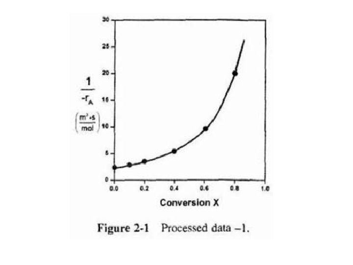
For this first-order dependence, a plot of reciprocal rate of reaction (1/-r. A) as a function of X yields a curve similar to one shown in Figure 2 -1. where

To illustrate design of a series of reactors, we consider isothermal gas-phase isomerization We are going to laboratory to determine rate of chemical reaction as a function of X of reactant A.

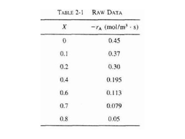
Table 2 -1 (laboratory measurements) show –r. A as a function of X. Temperature was 500 K (440°F), total pressure was 830 k. Pa (8. 2 atm), & initial charge to reactor was pure A.

For CSTR & PFR design equations, (2 -13) & (2 -16), reactor volume varies with reciprocal of –r. A. Consequently, to size reactors, convert rate data in Table 2 -1 to reciprocal rates in Table 22:

These data are used to arrive at a plot of (1/-r. A) as a function of X, shown in Fig. (2 -1).

Use this figure to size flow reactors for different entering molar flow rates. Before sizing flow reactors let's first consider some insights.

If a reaction is carried out isothermally, rate is usually greatest at start of reaction when concentration of reactant is greatest (i. e. , when there is negligible conversion [X≈0]). Hence (1/-r. A) will be small.

Near end of reaction, when reactant has been mostly used up & thus concentration of A is small (i. e. , conversion is large), reaction rate will be small. Consequently, (1/r. A) is large.

For all irreversible reactions of greater than zero order, as we approach complete conversion where all limiting reactant is used up, i. e. , X = 1, reciprocal rate approaches infinity as does reactor volume, i. e.

For reversible reactions, maximum conversion is equilibrium conversion Xe. At equilibrium, reaction rate is zero (r. A=0). Therefore,

To size a number of reactors for reaction, use FA 0= 0. 4 mol/s (calculated in Example 2 -1) to add another row to processed data shown in Table 2 -2 to obtain Table 2 -3.

8 -2 -2010

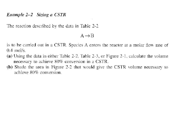
Solution: a) Eq. (2 -13) gives volume of a CSTR

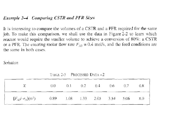
b) Shade area in Figure 2 -2 that yields CSTR volume. Rearranging Eq. (2 - 13) gives In Fig. E 2 -2. 1, volume is equal to area of a rectangle with a height (FA 0/-r. A=8 m 3) & a base (X= 0. 81).

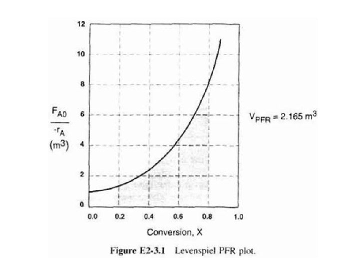
Solution start by repeating rows ( 1 ) & (4) of Table 2 -3. a) For PFR Five point quadrature formula (A-23) given in Appendix A. 4 to solve numerically above Eq.

Four equal segments between X = 0 & X = 0. 8 with a segment length of ▲X=0. 8/4 = 0. 2

b) Integral in Eq. (2 -16) can also be evaluated from area under curve of a plot of (FA/-r. A) versus X. For 80% conversion, shaded area 3 is roughly equal to 2165 dm (2. 165 m 3).

c) For X = 0. 2, calculate corresponding reactor volume using Simpson’s rule (given in Appendix A. 4 as Equation [A 21]) with ▲X = 0. 1 & data in rows 1 & 4 in Table 2 -3,

We can continue in this manner to arrive at Table E 2 -3. 1.

Data in Table E 1 -3. 1 are plotted in Figures E 2 -3. 2 (a) & (b).

When we combine Figs. E 2 -2. 1 & E 2 -3. 1 on same graph, we see that crosshatched area above curve is difference in CSTR & PFR reactor volumes.

For isothermal reactions greater than zero order, CSTR volume will usually be greater than PFR volume for same X & reaction conditions (temperature, Bow rate, etc. ).

We see that reason isothermal CSTR volume is usually greater than PFR volume is that CSTR is always operating at lowest reaction rate (e. g. , -r. A= 0. 05 in Figure E 2 -4. 1(b)).

PFR on other hand starts at a high rate at entrance & gradually decreases to exit rate, thereby requiring less volume because volume is inversely proportional to rate.

2. 5 Reactors in Series Many times, reactors are connected in series so that exit stream of one reactor is feed stream for another reactor. When this arrangement is used, it is often possible to speed calculations by defining conversion in terms of location at a point downstream rather than with respect to any single reactor.

That is, X is total number of moles of A that have reacted up to that point per mole of A fed to first reactor. For reactors in series

However, this definition can only be used when feed stream only enters first reactor in series & there are no side streams either fed or withdrawn. Molar flow rate of A at point i is equal to moles of A fed to first reactor minus all the moles of A reacted up to point i:

For reactors shown in Figure 2 -3, X 1 at point i = 1 is conversion achieved in PFR, X 2 at point i = 2 is total conversion achieved at this point in PFR & CSTR, & X 3 is total conversion achieved by all three reactors.

To demonstrate these ideas, let us consider three different schemes of reactors in series: two CSTRs, two PFRs. & then a combination of PFRs & CSTRs in series. To size these reactors, use laboratory data that gives reaction rate at different conversions.

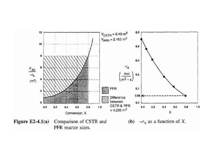
2. 5. 1 CSTRs in Series First scheme to be considered is two CSTRs in series shown in Figure 2 -4.

1 st reactor, rate of disappearance of A is r. A at X 1. A mole balance on reactor 1 gives molar flow rate of A at point 1 is Combining Equations (2 -19) & (2 -20) & rearranging

2 nd reactor, rate of disappearance of A, r. A 2, evaluated at conversion of exit stream of reactor 2, X 2, A mole balance on second reactor molar flow rate of A at point 2 is

Combining & rearranging For 2 nd CSTR recall that –r. A 2 is evaluated at X 2 &then use (X 2 -X 1) to calculate V 2 at X 2.

Example 2 -5 Comparing Volumes for CSTRs in Series For 2 CSTRs in series, 40% conversion is achieved in 1 st reactor. What is volume of each of two reactors necessary to achieve 80% overall conversion of entering species A?

Solution For 1 st reactor, we observe from either Table 2 -3 or Fig. E 2 -5. l that when X= 0. 4, then

For 2 nd reactor, when X 2 = 0. 8, then

Note again that for CSTRs in series, rate –r. A 1 is evaluated at a X of 0. 4 & rate – r. A 2 is evaluated at a X of 0. 8. Total volume for these two reactors in series is By comparison, volume necessary to achieve 80% conversion in one CSTR is

In Example 2 -5 that sum of two CSTR reactor 3 volumes (4. 02 m ) in series is less than volume 3 of one CSTR (6. 4 m ) to achieve same conversion.

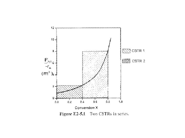
Approximating a PFR by a large number of CSTRs in series Consider approximating a PFR with a number of small, equal-volume CSTRs of Vi; in series (Fig. 2 -5). We want to compare total volume of all CSTRs with volume of one plugflow reactor for same conversion, say 80%.

From Fig. 2 -6, a very important observation! Total volume to achieve 80% conversion for five CSTRs of equal volume in series is roughly same as volume of a PFR.

As we make volume of each CSTR smaller & increase number of CSTRs, total volume of CSTRs in series & volume of PFR will become identical. That is, we can model a PFR with a large number of CSTRs in series.

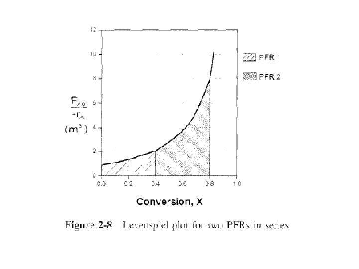
2. 5. 2 PFRs in Series We saw that 2 CSTRs in series gave a smaller total volume than a single CSTR to achieve same X. This case does not hold true for two plug-flow reactors connected in series shown in Fig. 2 -7.

We can see from Fig. 2 -8 & from following equation: that it is immaterial whether you place 2 plugflow reactors in series or have one continuous plug-flow reactor; total reactor volume required to achieve same conversion is identical.

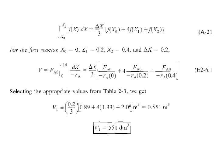
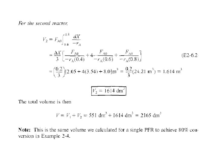
Example 2 -6 Sizing Plug-Flow Reactors in Series Using either data in Table 2 -3 or Fig. 2 -2, calculate reactor volumes V 1 & V 2 for plug-flow sequence shown in Fig. 2 -7 when intermediate conversion is 40% & final conversion is 80%.

Solution In addition to graphical integration, we could have used numerical methods to size plugflow reactors. Use Simpson’s rule (see Appendix A. 4) to evaluate integrals.

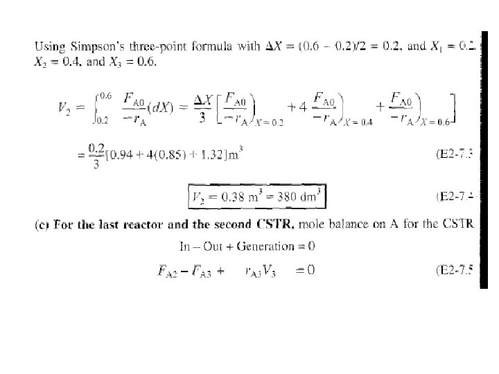
2. 5. 3 Combinations of CSTRs & PFRs in Series Final sequences, consider combinations of CSTRs & PFRs in series.

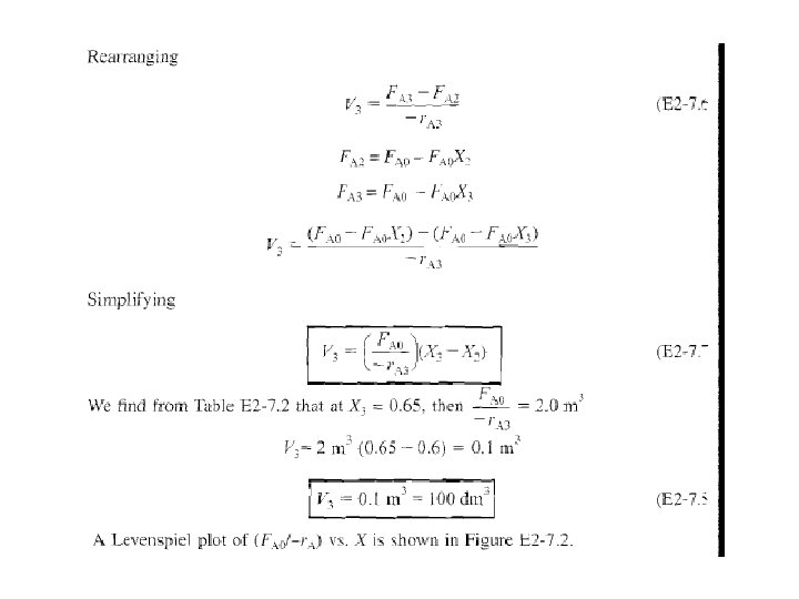
A schematic is shown in Fig. 2 -10.

Rearranging & integrating between limits, when V = 0, then X = X 2, & when V =V 3, then X =X 3.

The corresponding reactor volumes for each of three reactors can be found from shaded areas in Fig. 2 -11.

The FA 0/-r. A curves we have been using in previous examples are typical of those found in isothermal reaction systems.

Now consider a real reaction system that is carried out adiabatically. Isothermal reaction systems are discussed in Chapter 4 & adiabatic systems in Chapter 8.

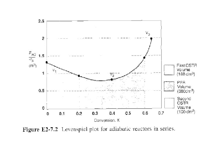
Example 2 -7 An Adiabatic Liquid. Phase Isomerization of butane was carried out adiabatically in liquid phase & data in Table E 2 -7. 1 were obtained.

It is real data for a real reaction carried out adiabatically, & reactor scheme shown in Fig. E 2 -7. 1 is used.

Calculate volume of each of reactors for an entering molar flow rate of nbutane of 50 kmol/hr.

Solution

2. 5. 4 Comparing CSTR & PFR Reactor Volumes & Reactor Sequencing Look at Fig. E 2 -7. 2, area under curve (PFR volume) between X = 0 & X = 0. 2, PFR area is greater than rectangular area corresponding to CSTR volume, i. e. , VPFR>VCSTR.

However, if we compare areas under curve between X = 0. 6 & X = 0. 65, area under curve (PFR volume) is smaller than rectangular area corresponding to the CSTR volume, i. e. , VCSTR > VPFR.

In sequencing of reactors one is often asked, “Which reactor should go first to give highest overall conversion? Should it be a PFR followed by a CSTR, or two CSTRs, then a PFR, or. . . ? ”

Answer is “It depends. ”It depends not only on shape of Levenspiel plots (FA 0/-r. A) versus X, but also on relative reactor sizes.

As an exercise, examine Figure E 2 -7. 2 to learn if there is a better way to arrange two CSTRs & one PFR. Suppose you were given a Levenspiel plot of (FA 0/-r. A) vs. X for three reactors in series along with their reactor volumes VCSTR 1= 3 m 3, VCSTR 2 = 2 m 3, & VPFR = 1. 2 m 3 & asked to find highest possible conversion X.

What would you do? The methods we used to calculate reactor volumes all apply, except procedure is reversed & a trial-and-error solution is needed to find exit overall conversion from each reactor.

Previous examples show that if we know molar flow rate to reactor & reaction rate as a function of conversion, then we can calculate reactor volume necessary to achieve a specified conversion.

Reaction rate does not depend on conversion alone, however, it is also affected by initial concentrations of reactants, temperature, & pressure.

It is important to understand that if rate of reaction is available or can be obtained solely as a function of conversion, -r. A = f(X), or if can be generated by some intermediate calculations, one can design a variety of reactors or a combination of reactors.

2. 6 Some Further Definitions Before proceeding to Chapter 3, some terms & equations commonly used in reaction engineering need to be defined. Consider special case or plug-flow design equation when volumetric flow rate is constant.

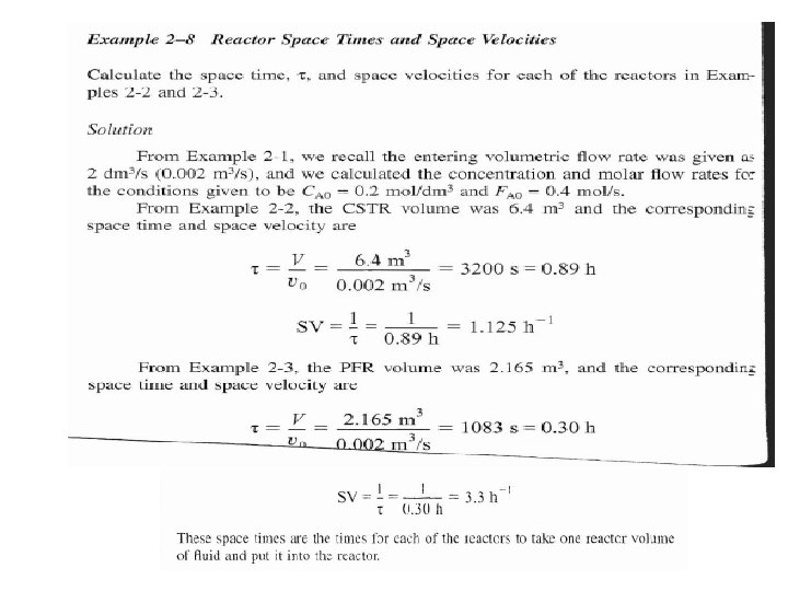
2. 6. 1 Space Time Space time, τ, is obtained by dividing reactor volume by volumetric flow rate entering reactor:

Space time is time necessary to process one reactor volume of fluid based on entrance conditions. For example, consider tubular reactor shown in Fig. 2 -12, which 3 is 20 m long & 0. 2 m in volume.

The dashed line in Figure 2 -12 represents 0. 2 m 3 of fluid directly upstream of reactor. Time it takes for this fluid to enter reactor completely is space time. It is also called holding time or mean residence time.

For example, if volumetric flow rate were 0. 01 m 3/s, take upstream volume shown by dashed lines a time τ to enter reactor. In other words, it would take 20 s for fluid at point a to move to point b, which corresponds to a space time of 20 s.

2. 6. 2 Space Velocity Sspace velocity (SV), which is defined as might be regarded at first sight as reciprocal of space time. However, there can be a difference in two quantities definitions. For space time, entering volumetric flow rate is measured at entrance conditions, but for space velocity, other conditions are often used.

Two space velocities commonly used in industry are liquidhourly & gas-hourly space velocities, LHSV & GHSV, respectively.

Entering volumetric flow rate, ν 0, in LHSV is frequently measured as that of a liquid feed rate at 600 F or 750 F, even though feed to reactor may be a vapor at some higher temperature. Gas volumetric flow rate, ν 0, in GHSV is normally measured at standard temperature & pressure (STP).