Chapter TwentyOne Multidimensional Scaling and Conjoint Analysis 21

Chapter Twenty-One Multidimensional Scaling and Conjoint Analysis

21 -2 Chapter Outline 1) Overview 2) Basic Concepts in Multidimensional Scaling (MDS) 3) Statistics & Terms Associated with MDS

21 -3 Chapter Outline 4) Conducting Multidimensional Scaling i. Formulating the Problem ii. Obtaining Input Data a. Perception Data: Direct Approaches b. Perception Data: Derived Approaches c. Direct Vs. Derived Approaches d. Preference Data iii. Selecting an MDS Procedure iv. Deciding on the Number of Dimensions v. Labeling the Dimensions & Interpreting the Configuration vi. Assessing Reliability and Validity

21 -4 Chapter Outline 5) Assumptions & Limitations of MDS 6) Scaling Preference Data 7) Correspondence Analysis 8) Relationship between MDS, Factor Analysis, & Discriminant Analysis 9) Basic Concepts in Conjoint Analysis 10) Statistics & Terms Associated with Conjoint Analysis

21 -5 Chapter Outline 11) Conducting Conjoint Analysis i. Formulating the Problem ii. Constructing the Stimuli iii. Deciding on the Form of Input Data iv. Selecting a Conjoint Analysis Procedure v. Interpreting the Results vi. Assessing Reliability and Validity 12) Assumptions & Limitations of Conjoint Analysis 13) Hybrid Conjoint Analysis

21 -6 Chapter Outline 14) Internet & Computer Applications 15) Focus on Burke 16) Summary 17) Key Terms and Concepts

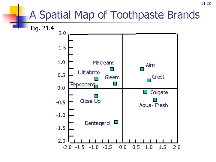
21 -7 Multidimensional Scaling (MDS) n n n Multidimensional scaling (MDS) is a class of procedures for representing perceptions and preferences of respondents spatially by means of a visual display. Perceived or psychological relationships among stimuli are represented as geometric relationships among points in a multidimensional space. These geometric representations are often called spatial maps. The axes of the spatial map are assumed to denote the psychological bases or underlying dimensions respondents use to form perceptions and preferences for stimuli.

21 -8 Statistics and Terms Associated with MDS n n Similarity judgments are ratings on all possible pairs of brands or other stimuli in terms of their similarity using a Likert type scale. Preference rankings are rank orderings of the brands or other stimuli from the most preferred to the least preferred. They are normally obtained from the respondents. Stress. This is a lack-of-fit measure; higher values of stress indicate poorer fits. R-square is a squared correlation index that indicates the proportion of variance of the optimally scaled data that can be accounted for by the MDS procedure. This is a goodness-of-fit measure.

21 -9 Statistics and Terms Associated with MDS n n n Spatial map. Perceived relationships among brands or other stimuli are represented as geometric relationships among points in a multidimensional space called a spatial map. Coordinates indicate the positioning of a brand or a stimulus in a spatial map. Unfolding. The representation of both brands and respondents as points in the same space is referred to as unfolding.

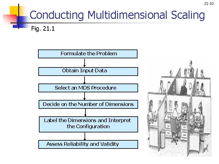
21 -10 Conducting Multidimensional Scaling Fig. 21. 1 Formulate the Problem Obtain Input Data Select an MDS Procedure Decide on the Number of Dimensions Label the Dimensions and Interpret the Configuration Assess Reliability and Validity

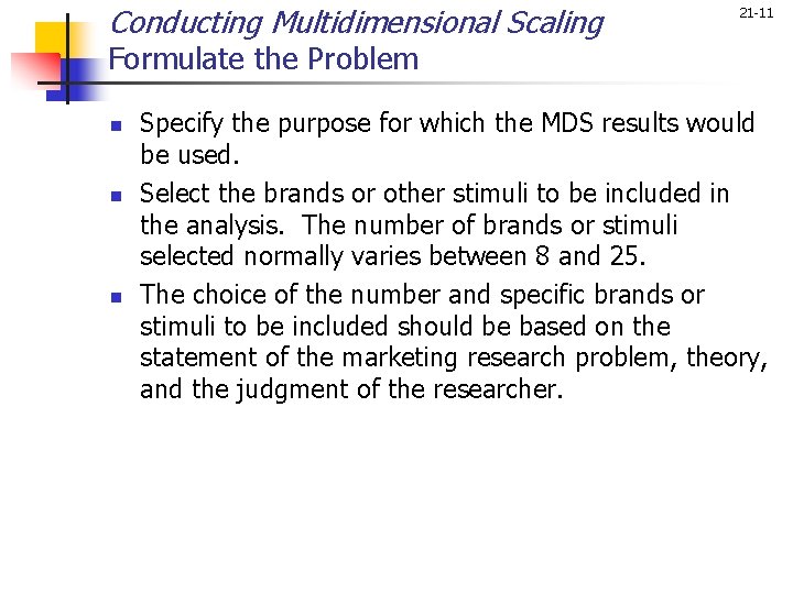
Conducting Multidimensional Scaling 21 -11 Formulate the Problem n n n Specify the purpose for which the MDS results would be used. Select the brands or other stimuli to be included in the analysis. The number of brands or stimuli selected normally varies between 8 and 25. The choice of the number and specific brands or stimuli to be included should be based on the statement of the marketing research problem, theory, and the judgment of the researcher.

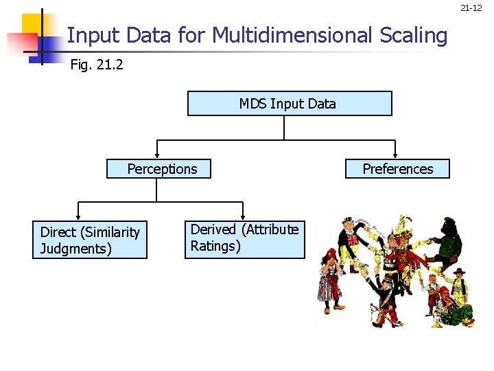
21 -12 Input Data for Multidimensional Scaling Fig. 21. 2 MDS Input Data Perceptions Direct (Similarity Judgments) Derived (Attribute Ratings) Preferences

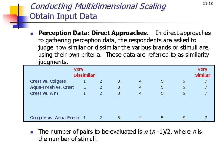
Conducting Multidimensional Scaling 21 -13 Obtain Input Data n Perception Data: Direct Approaches. In direct approaches to gathering perception data, the respondents are asked to judge how similar or dissimilar the various brands or stimuli are, using their own criteria. These data are referred to as similarity judgments. Very Dissimilar Crest vs. Colgate 1 Aqua-Fresh vs. Crest 1 Crest vs. Aim 1. . . Colgate vs. Aqua-Fresh 1 n 2 2 2 3 3 3 4 4 4 5 5 5 6 6 6 2 3 4 5 6 Very Similar 7 7 7 The number of pairs to be evaluated is n (n -1)/2, where n is the number of stimuli. 7

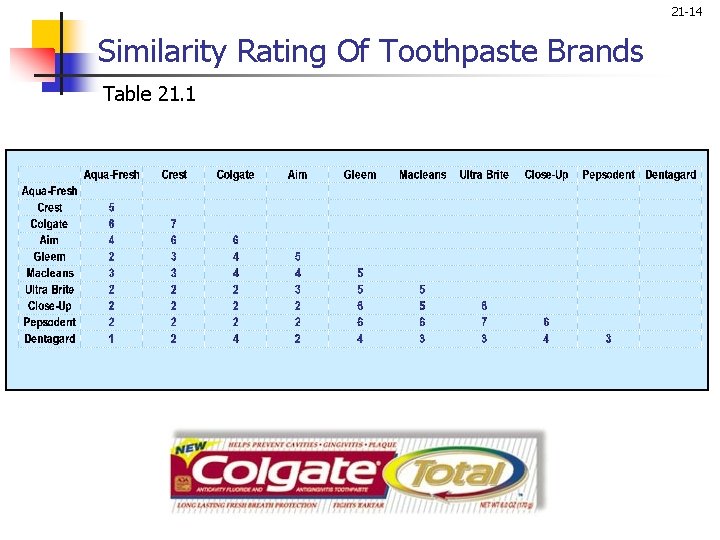
21 -14 Similarity Rating Of Toothpaste Brands Table 21. 1

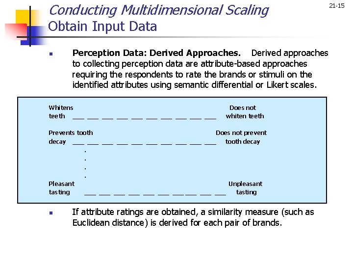
Conducting Multidimensional Scaling Obtain Input Data n Perception Data: Derived Approaches. Derived approaches to collecting perception data are attribute-based approaches requiring the respondents to rate the brands or stimuli on the identified attributes using semantic differential or Likert scales. Whitens teeth ___ ___ ___ Does not whiten teeth Prevents tooth Does not prevent decay ___ ___ ___ tooth decay. . Pleasant Unpleasant tasting ___ ___ ___ tasting n If attribute ratings are obtained, a similarity measure (such as Euclidean distance) is derived for each pair of brands. 21 -15

Conducting Multidimensional Scaling 21 -16 Obtain Input Data – Direct vs. Derived Approaches The direct approach has the following advantages and disadvantages: n The researcher does not have to identify a set of salient attributes. n The disadvantages are that the criteria are influenced by the brands or stimuli being evaluated. n Furthermore, it may be difficult to label the dimensions of the spatial map.

Conducting Multidimensional Scaling 21 -17 Obtain Input Data – Direct vs. Derived Approaches The attribute-based approach has the following advantages and disadvantages: n It is easy to identify respondents with homogeneous perceptions. n The respondents can be clustered based on the attribute ratings. n It is also easier to label the dimensions. n A disadvantage is that the researcher must identify all the salient attributes, a difficult task. n The spatial map obtained depends upon the attributes identified. It may be best to use both these approaches in a complementary way. Direct similarity judgments may be used for obtaining the spatial map, and attribute ratings may be used as an aid to interpreting the dimensions of the perceptual map.

Conducting Multidimensional Scaling 21 -18 Preference Data n n n Preference data order the brands or stimuli in terms of respondents' preference for some property. A common way in which such data are obtained is through preference rankings. Alternatively, respondents may be required to make paired comparisons and indicate which brand in a pair they prefer. Another method is to obtain preference ratings for the various brands. The configuration derived from preference data may differ greatly from that obtained from similarity data. Two brands may be perceived as different in a similarity map yet similar in a preference map, and vice versa. .

Conducting Multidimensional Scaling 21 -19 Select an MDS Procedure Selection of a specific MDS procedure depends upon: n Whether perception or preference data are being scaled, or whether the analysis requires both kinds of data. n The nature of the input data is also a determining factor. n Non-metric MDS procedures assume that the input data are ordinal, but they result in metric output. n Metric MDS methods assume that input data are metric. Since the output is also metric, a stronger relationship between the output and input data is maintained, and the metric (interval or ratio) qualities of the input data are preserved. n The metric and non-metric methods produce similar results. n Another factor influencing the selection of a procedure is whether the MDS analysis will be conducted at the individual respondent level or at an aggregate level.

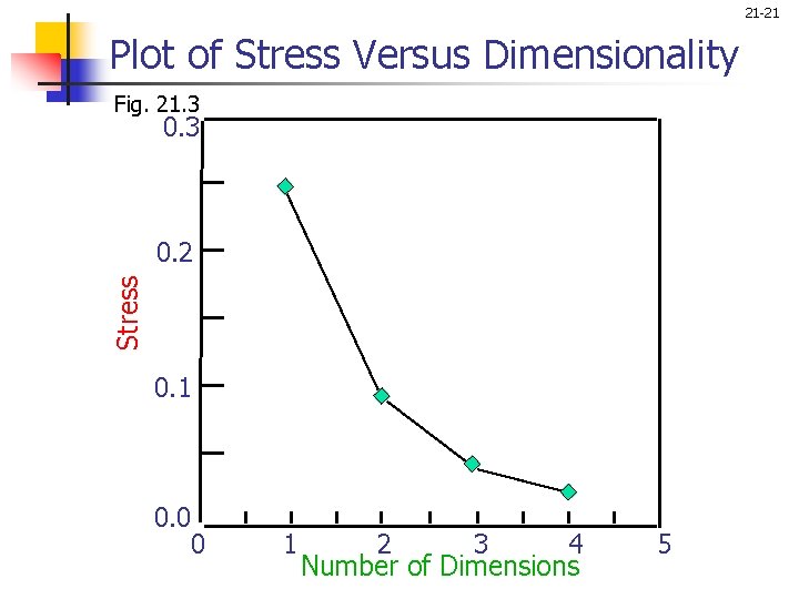
Conducting Multidimensional Scaling 21 -20 Decide on the Number of Dimensions n n n A priori knowledge - Theory or past research may suggest a particular number of dimensions. Interpretability of the spatial map - Generally, it is difficult to interpret configurations or maps derived in more than three dimensions. Elbow criterion - A plot of stress versus dimensionality should be examined. Ease of use - It is generally easier to work with twodimensional maps or configurations than with those involving more dimensions. Statistical approaches - For the sophisticated user, statistical approaches are also available for determining the dimensionality.

21 -21 Plot of Stress Versus Dimensionality Fig. 21. 3 0. 3 Stress 0. 2 0. 1 0. 0 0 1 2 3 4 Number of Dimensions 5

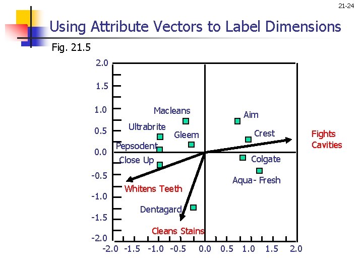
Conducting Multidimensional Scaling 21 -22 Label the Dimensions and Interpret the Configuration n n Even if direct similarity judgments are obtained, ratings of the brands on researcher-supplied attributes may still be collected. Using statistical methods such as regression, these attribute vectors may be fitted in the spatial map. After providing direct similarity or preference data, the respondents may be asked to indicate the criteria they used in making their evaluations. If possible, the respondents can be shown their spatial maps and asked to label the dimensions by inspecting the configurations. If objective characteristics of the brands are available (e. g. , horsepower or miles per gallon for automobiles), these could be used as an aid in interpreting the subjective dimensions of the spatial maps.

21 -23 A Spatial Map of Toothpaste Brands Fig. 21. 4 2. 0 1. 5 1. 0 0. 5 0. 0 -0. 5 Macleans Ultrabrite Aim Gleem Crest Pepsodent Colgate Close Up Aqua- Fresh -1. 0 -1. 5 Dentagard -2. 0 -1. 5 -1. 0 -0. 5 0. 0 0. 5 1. 0 1. 5 2. 0

21 -24 Using Attribute Vectors to Label Dimensions Fig. 21. 5 2. 0 1. 5 1. 0 0. 5 0. 0 Macleans Ultrabrite -1. 5 Crest Gleem Fights Cavities Pepsodent Colgate Close Up -0. 5 -1. 0 Aim Whitens Teeth Aqua- Fresh Dentagard Cleans Stains -2. 0 -1. 5 -1. 0 -0. 5 0. 0 0. 5 1. 0 1. 5 2. 0

Conducting Multidimensional Scaling 21 -25 Assess Reliability and Validity n n n The index of fit, or R-square is a squared correlation index that indicates the proportion of variance of the optimally scaled data that can be accounted for by the MDS procedure. Values of 0. 60 or better are considered acceptable. Stress values are also indicative of the quality of MDS solutions. While R-square is a measure of goodness-of-fit, stress measures badness-of-fit, or the proportion of variance of the optimally scaled data that is not accounted for by the MDS model. Stress values of less than 10% are considered acceptable. If an aggregate-level analysis has been done, the original data should be split into two or more parts. MDS analysis should be conducted separately on each part and the results compared.

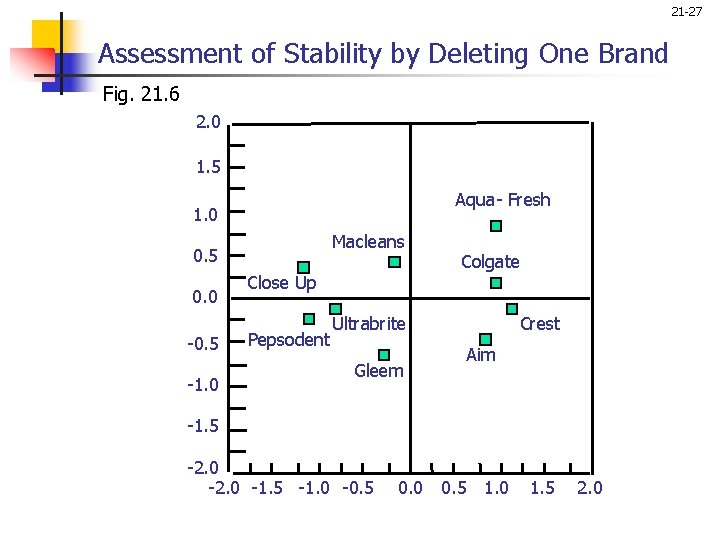
Conducting Multidimensional Scaling 21 -26 Assess Reliability and Validity n n n Stimuli can be selectively eliminated from the input data and the solutions determined for the remaining stimuli. A random error term could be added to the input data. The resulting data are subjected to MDS analysis and the solutions compared. The input data could be collected at two different points in time and the test-retest reliability determined.

21 -27 Assessment of Stability by Deleting One Brand Fig. 21. 6 2. 0 1. 5 Aqua- Fresh 1. 0 Macleans 0. 5 0. 0 -0. 5 -1. 0 Close Up Pepsodent Colgate Ultrabrite Gleem Crest Aim -1. 5 -2. 0 -1. 5 -1. 0 -0. 5 0. 0 0. 5 1. 0 1. 5 2. 0

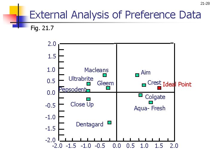
21 -28 External Analysis of Preference Data Fig. 21. 7 2. 0 1. 5 1. 0 Macleans Ultrabrite 0. 5 Gleem Pepsodent 0. 0 -0. 5 -1. 0 -1. 5 Close Up Aim Crest Ideal Point Colgate Aqua- Fresh Dentagard -2. 0 -1. 5 -1. 0 -0. 5 0. 0 0. 5 1. 0 1. 5 2. 0

21 -29 Assumptions and Limitations of MDS n n It is assumed that the similarity of stimulus A to B is the same as the similarity of stimulus B to A. MDS assumes that the distance (similarity) between two stimuli is some function of their partial similarities on each of several perceptual dimensions. When a spatial map is obtained, it is assumed that interpoint distances are ratio scaled and that the axes of the map are multidimensional interval scaled. A limitation of MDS is that dimension interpretation relating physical changes in brands or stimuli to changes in the perceptual map is difficult at best.

21 -30 Scaling Preference Data n n In internal analysis of preferences, a spatial map representing both brands or stimuli and respondent points or vectors is derived solely from the preference data. In external analysis of preferences, the ideal points or vectors based on preference data are fitted in a spatial map derived from perception (e. g. , similarities) data. The representation of both brands and respondents as points in the same space, by using internal or external analysis, is referred to as unfolding. External analysis is preferred in most situations.

21 -31 Correspondence Analysis n n Correspondence analysis is an MDS technique for scaling qualitative data in marketing research. The input data are in the form of a contingency table, indicating a qualitative association between the rows and columns. Correspondence analysis scales the rows and columns in corresponding units, so that each can be displayed graphically in the same low-dimensional space. These spatial maps provide insights into (1) similarities and differences within the rows with respect to a given column category; (2) similarities and differences within the column categories with respect to a given row category; and (3) relationship among the rows and columns.

21 -32 Correspondence Analysis n n n The advantage of correspondence analysis, as compared to other multidimensional scaling techniques, is that it reduces the data collection demands imposed on the respondents, since only binary or categorical data are obtained. The disadvantage is that between set (i. e. , between column and row) distances cannot be meaningfully interpreted. Correspondence analysis is an exploratory data analysis technique that is not suitable for hypothesis testing.

Relationship Among MDS, Factor Analysis, and Discriminant Analysis n n n 21 -33 If the attribute-based approaches are used to obtain input data, spatial maps can also be obtained by using factor or discriminant analysis. By factor analyzing the data, one could derive for each respondent, factor scores for each brand. By plotting brand scores on the factors, a spatial map could be obtained for each respondent. The dimensions would be labeled by examining the factor loadings, which are estimates of the correlations between attribute ratings and underlying factors. To develop spatial maps by means of discriminant analysis, the dependent variable is the brand rated and the independent or predictor variables are the attribute ratings. A spatial map can be obtained by plotting the discriminant scores for the brands. The dimensions can be labeled by examining the discriminant weights, or the weightings of attributes that make up a discriminant function or dimension.

21 -34 Conjoint Analysis n n n Conjoint analysis attempts to determine the relative importance consumers attach to salient attributes and the utilities they attach to the levels of attributes. The respondents are presented with stimuli that consist of combinations of attribute levels and asked to evaluate these stimuli in terms of their desirability. Conjoint procedures attempt to assign values to the levels of each attribute, so that the resulting values or utilities attached to the stimuli match, as closely as possible, the input evaluations provided by the respondents.

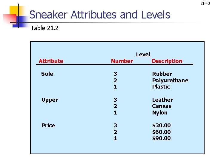
Statistics and Terms Associated with Conjoint Analysis n n n 21 -35 Part-worth functions. The part-worth functions, or utility functions, describe the utility consumers attach to the levels of each attribute. Relative importance weights. The relative importance weights are estimated and indicate which attributes are important in influencing consumer choice. Attribute levels. The attribute levels denote the values assumed by the attributes. Full profiles, or complete profiles of brands, are constructed in terms of all the attributes by using the attribute levels specified by the design. Pairwise tables. In pairwise tables, the respondents evaluate two attributes at a time until all the required pairs of attributes have been evaluated.

Statistics and Terms Associated with Conjoint Analysis n n 21 -36 Cyclical designs are designs employed to reduce the number of paired comparisons. Fractional factorial designs are designs employed to reduce the number of stimulus profiles to be evaluated in the full profile approach. Orthogonal arrays are a special class of fractional designs that enable the efficient estimation of all main effects. Internal validity. This involves correlations of the predicted evaluations for the holdout or validation stimuli with those obtained from the respondents.

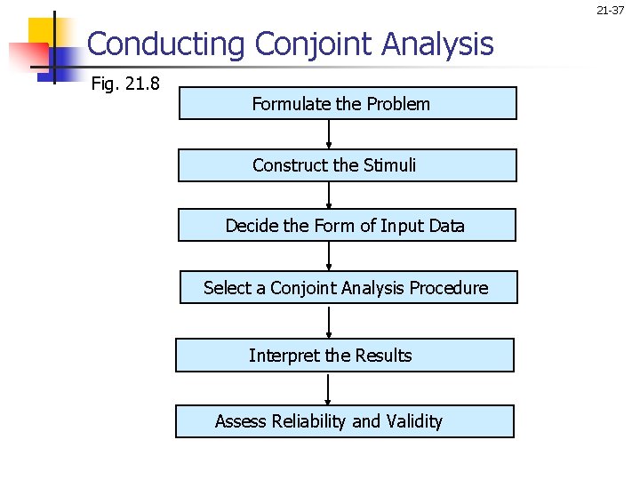
21 -37 Conducting Conjoint Analysis Fig. 21. 8 Formulate the Problem Construct the Stimuli Decide the Form of Input Data Select a Conjoint Analysis Procedure Interpret the Results Assess Reliability and Validity

Conducting Conjoint Analysis 21 -38 Formulate the Problem n n n Identify the attributes and attribute levels to be used in constructing the stimuli. The attributes selected should be salient in influencing consumer preference and choice and should be actionable. A typical conjoint analysis study involves six or seven attributes. At least three levels should be used, unless the attribute naturally occurs in binary form (two levels). The researcher should take into account the attribute levels prevalent in the marketplace and the objectives of the study.

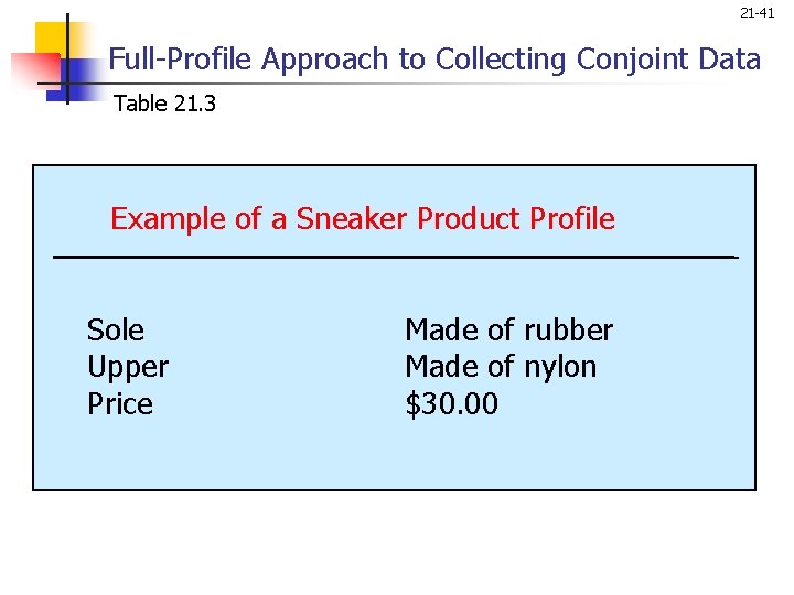
Conducting Conjoint Analysis 21 -39 Construct the Stimuli n n n In the pairwise approach, also called two-factor evaluations, the respondents evaluate two attributes at a time until all the possible pairs of attributes have been evaluated. In the full-profile approach, also called multiplefactor evaluations, full or complete profiles of brands are constructed for all the attributes. Typically, each profile is described on a separate index card. In the pairwise approach, it is possible to reduce the number of paired comparisons by using cyclical designs. Likewise, in the full-profile approach, the number of stimulus profiles can be greatly reduced by means of fractional factorial designs.

21 -40 Sneaker Attributes and Levels Table 21. 2 Attribute Number Level Description Sole 3 2 1 Rubber Polyurethane Plastic Upper 3 2 1 Leather Canvas Nylon Price 3 2 1 $30. 00 $60. 00 $90. 00

21 -41 Full-Profile Approach to Collecting Conjoint Data Table 21. 3 Example of a Sneaker Product Profile Sole Upper Price Made of rubber Made of nylon $30. 00

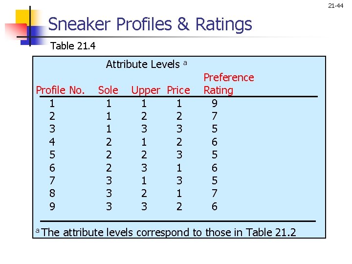
Conducting Conjoint Analysis 21 -42 Construct the Stimuli n n A special class of fractional designs, called orthogonal arrays, allow for the efficient estimation of all main effects. Orthogonal arrays permit the measurement of all main effects of interest on an uncorrelated basis. These designs assume that all interactions are negligible. Generally, two sets of data are obtained. One, the estimation set, is used to calculate the part-worth functions for the attribute levels. The other, the holdout set, is used to assess reliability and validity.

Conducting Conjoint Analysis 21 -43 Decide on the Form of Input Data n n n For non-metric data, the respondents are typically required to provide rank-order evaluations. In the metric form, the respondents provide ratings, rather than rankings. In this case, the judgments are typically made independently. In recent years, the use of ratings has become increasingly common. The dependent variable is usually preference or intention to buy. However, the conjoint methodology is flexible and can accommodate a range of other dependent variables, including actual purchase or choice. In evaluating sneaker profiles, respondents were required to provide preference.

21 -44 Sneaker Profiles & Ratings Table 21. 4 Attribute Levels Profile No. 1 2 3 4 5 6 7 8 9 a Sole 1 1 1 2 2 2 3 3 3 a Upper Price 1 1 2 2 3 3 1 1 3 2 Preference Rating 9 7 5 6 5 7 6 The attribute levels correspond to those in Table 21. 2

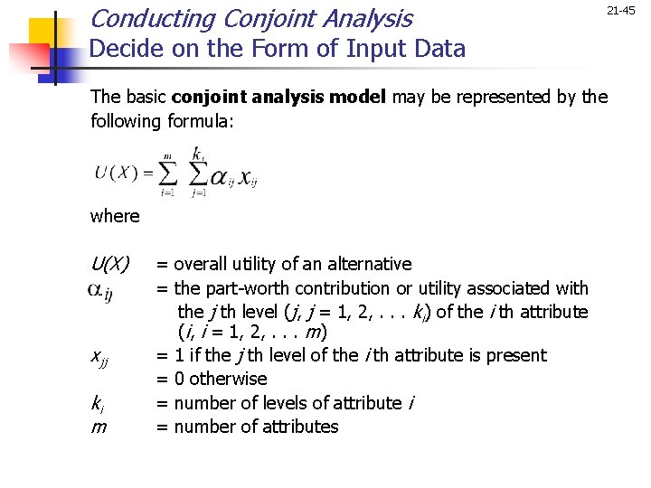
Conducting Conjoint Analysis 21 -45 Decide on the Form of Input Data The basic conjoint analysis model may be represented by the following formula: where U(X) xjj ki m = overall utility of an alternative = the part-worth contribution or utility associated with the j th level (j, j = 1, 2, . . . ki) of the i th attribute (i, i = 1, 2, . . . m) = 1 if the j th level of the i th attribute is present = 0 otherwise = number of levels of attribute i = number of attributes

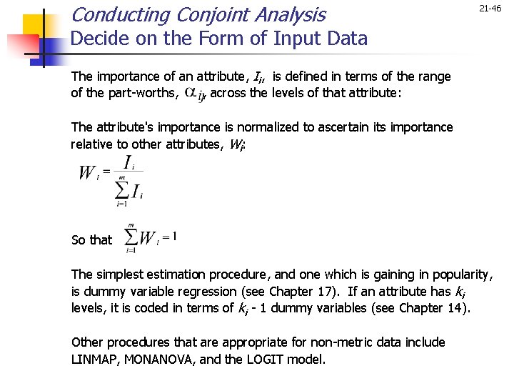
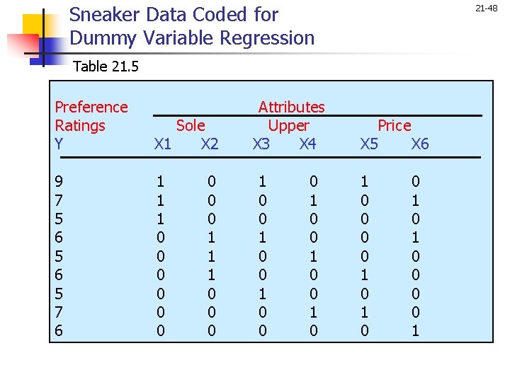
Conducting Conjoint Analysis 21 -46 Decide on the Form of Input Data The importance of an attribute, Ii, is defined in terms of the range of the part-worths, , across the levels of that attribute: The attribute's importance is normalized to ascertain its importance relative to other attributes, Wi: So that The simplest estimation procedure, and one which is gaining in popularity, is dummy variable regression (see Chapter 17). If an attribute has ki levels, it is coded in terms of ki - 1 dummy variables (see Chapter 14). Other procedures that are appropriate for non-metric data include LINMAP, MONANOVA, and the LOGIT model.

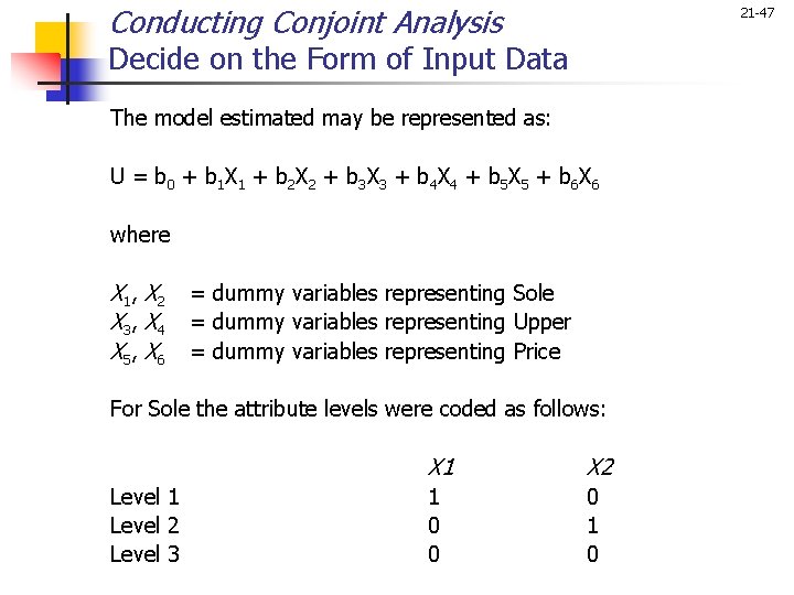
Conducting Conjoint Analysis 21 -47 Decide on the Form of Input Data The model estimated may be represented as: U = b 0 + b 1 X 1 + b 2 X 2 + b 3 X 3 + b 4 X 4 + b 5 X 5 + b 6 X 6 where X 1 , X 2 X 3 , X 4 X 5 , X 6 = dummy variables representing Sole = dummy variables representing Upper = dummy variables representing Price For Sole the attribute levels were coded as follows: Level 1 Level 2 Level 3 X 1 X 2 1 0 0 0 1 0

Sneaker Data Coded for Dummy Variable Regression 21 -48 Table 21. 5 Preference Ratings Y Sole X 1 X 2 9 7 5 6 5 7 6 1 1 1 0 0 0 0 0 1 1 1 0 0 0 Attributes Upper X 3 X 4 1 0 0 0 1 0 Price X 5 X 6 1 0 0 1 0 1 0 0 0 0 1

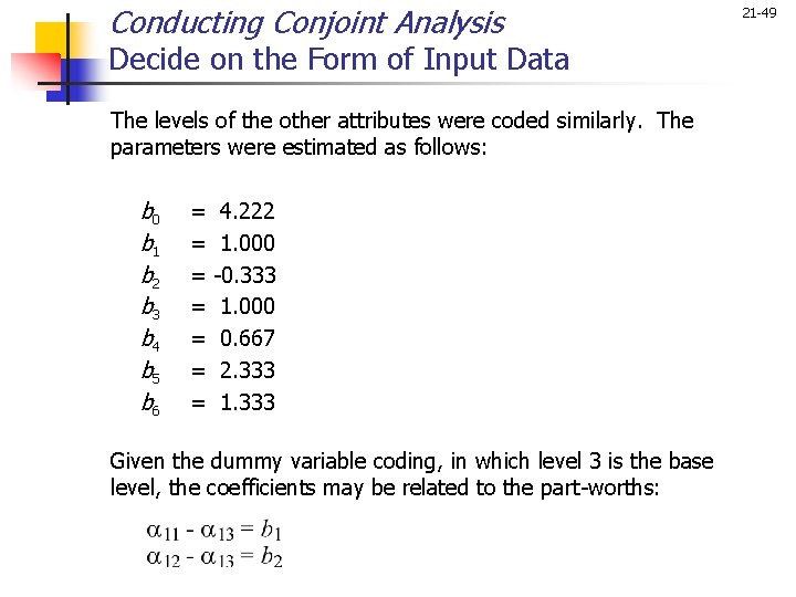
Conducting Conjoint Analysis Decide on the Form of Input Data The levels of the other attributes were coded similarly. The parameters were estimated as follows: b 0 b 1 b 2 b 3 b 4 b 5 b 6 = = = = 4. 222 1. 000 -0. 333 1. 000 0. 667 2. 333 1. 333 Given the dummy variable coding, in which level 3 is the base level, the coefficients may be related to the part-worths: 21 -49

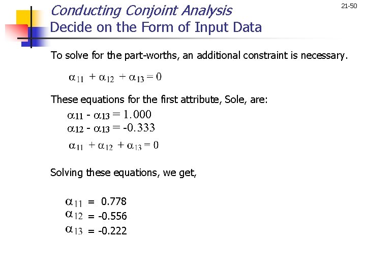
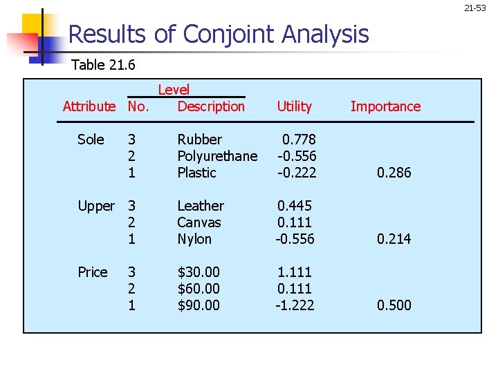
Conducting Conjoint Analysis 21 -50 Decide on the Form of Input Data To solve for the part-worths, an additional constraint is necessary. These equations for the first attribute, Sole, are: a 11 - a 13 = 1. 000 a 12 - a 13 = -0. 333 Solving these equations, we get, = 0. 778 = -0. 556 = -0. 222

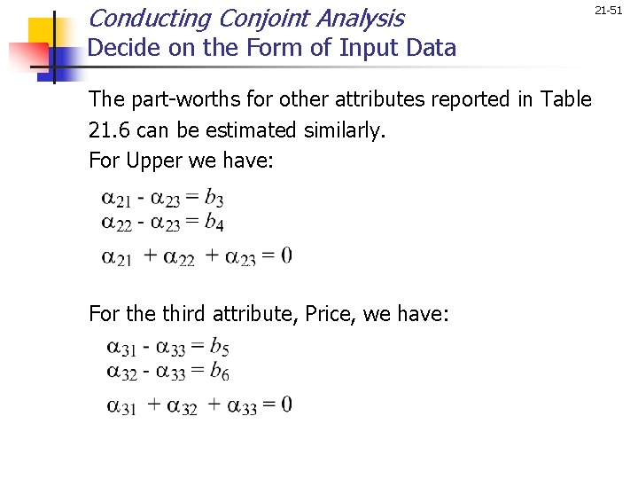
Conducting Conjoint Analysis Decide on the Form of Input Data The part-worths for other attributes reported in Table 21. 6 can be estimated similarly. For Upper we have: For the third attribute, Price, we have: 21 -51

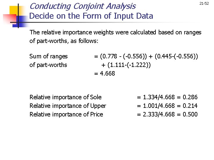
Conducting Conjoint Analysis 21 -52 Decide on the Form of Input Data The relative importance weights were calculated based on ranges of part-worths, as follows: Sum of ranges of part-worths = (0. 778 - (-0. 556)) + (0. 445 -(-0. 556)) + (1. 111 -(-1. 222)) = 4. 668 Relative importance of Sole Relative importance of Upper Relative importance of Price = 1. 334/4. 668 = 0. 286 = 1. 001/4. 668 = 0. 214 = 2. 333/4. 668 = 0. 500

21 -53 Results of Conjoint Analysis Table 21. 6 Level Attribute No. Description Sole 3 2 1 Utility Importance Rubber Polyurethane Plastic 0. 778 -0. 556 -0. 222 0. 286 Upper 3 2 1 Leather Canvas Nylon 0. 445 0. 111 -0. 556 0. 214 Price $30. 00 $60. 00 $90. 00 1. 111 0. 111 -1. 222 0. 500 3 2 1

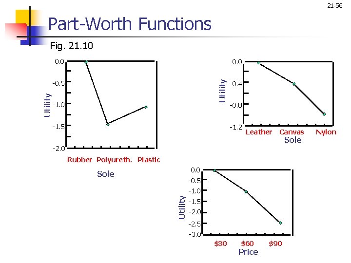
Conducting Conjoint Analysis 21 -54 Interpret the Results n n n For interpreting the results, it is helpful to plot the part-worth functions. The utility values have only interval scale properties, and their origin is arbitrary. The relative importance of attributes should be considered.

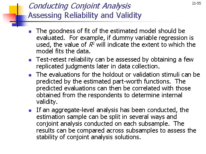
Conducting Conjoint Analysis 21 -55 Assessing Reliability and Validity n n The goodness of fit of the estimated model should be evaluated. For example, if dummy variable regression is used, the value of R 2 will indicate the extent to which the model fits the data. Test-retest reliability can be assessed by obtaining a few replicated judgments later in data collection. The evaluations for the holdout or validation stimuli can be predicted by the estimated part-worth functions. The predicted evaluations can then be correlated with those obtained from the respondents to determine internal validity. If an aggregate-level analysis has been conducted, the estimation sample can be split in several ways and conjoint analysis conducted on each subsample. The results can be compared across subsamples to assess the stability of conjoint analysis solutions.

21 -56 Part-Worth Functions Fig. 21. 10 0. 0 Utility 0. 0 -1. 5 -0. 4 -0. 8 -1. 2 Leather Canvas -2. 0 Rubber Polyureth. Plastic 0. 0 Sole -0. 5 -1. 0 Utility -0. 5 -1. 5 -2. 0 -2. 5 -3. 0 $30 $60 Price $90 Sole Nylon

Assumptions and Limitations of Conjoint Analysis n n n 21 -57 Conjoint analysis assumes that the important attributes of a product can be identified. It assumes that consumers evaluate the choice alternatives in terms of these attributes and make tradeoffs. The tradeoff model may not be a good representation of the choice process. Another limitation is that data collection may be complex, particularly if a large number of attributes are involved and the model must be estimated at the individual level. The part-worth functions are not unique.

21 -58 Hybrid Conjoint Analysis n n Hybrid models have been developed to serve two main purposes: 1. Simplify the data collection task by imposing less of a burden on each respondent, and 2. Permit the estimation of selected interactions (at the subgroup level) as well as all main (or simple) effects at the individual level. In the hybrid approach, the respondents evaluate a limited number, generally no more than nine, conjoint stimuli, such as full profiles.

21 -59 Hybrid Conjoint Analysis n n n These profiles are drawn from a large master design, and different respondents evaluate different sets of profiles, so that over a group of respondents, all the profiles of interest are evaluated. In addition, respondents directly evaluate the relative importance of each attribute and desirability of the levels of each attribute. By combining the direct evaluations with those derived from the evaluations of the conjoint stimuli, it is possible to estimate a model at the aggregate level and still retain some individual differences.

21 -60 SPSS Windows The multidimensional scaling program allows individual differences as well as aggregate analysis using ALSCAL. The level of measurement can be ordinal, interval or ratio. Both the direct and the derived approaches can be accommodated. To select multidimensional scaling procedures using SPSS for Windows click: Analyze>Scale>Multidimensional Scaling … The conjoint analysis approach can be implemented using regression if the dependent variable is metric (interval or ratio). This procedure can be run by clicking: Analyze>Regression>Linear …