Chapter Twenty Seven Theory of Active Portfolio Management

Chapter Twenty Seven Theory of Active Portfolio Management INVESTMENTS | BODIE, KANE, MARCUS © 2018 Mc. Graw-Hill Education. All rights reserved. Authorized only for instructor use in the classroom. No reproduction or further distribution permitted without the prior written consent of Mc. Graw-Hill Education.

Overview • Treynor-Black model • The optimization uses analysts’ forecasts of superior performance • The model is adjusted for tracking error and for analyst forecast error • Black-Litterman model • Quantify complex forecasts • Apply these views to portfolio construction INVESTMENTS | BODIE, KANE, MARCUS © 2018 Mc. Graw-Hill Education 27 -2

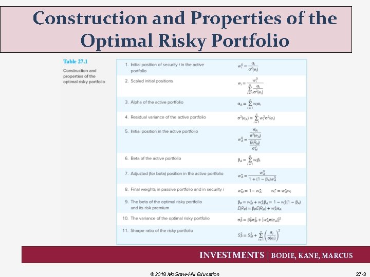
Construction and Properties of the Optimal Risky Portfolio INVESTMENTS | BODIE, KANE, MARCUS © 2018 Mc. Graw-Hill Education 27 -3

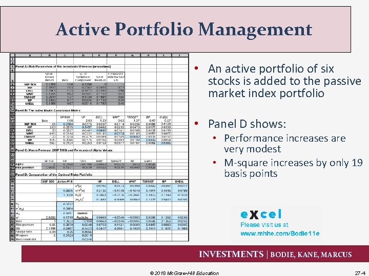
Active Portfolio Management • An active portfolio of six stocks is added to the passive market index portfolio • Panel D shows: • Performance increases are very modest • M-square increases by only 19 basis points INVESTMENTS | BODIE, KANE, MARCUS © 2018 Mc. Graw-Hill Education 27 -4

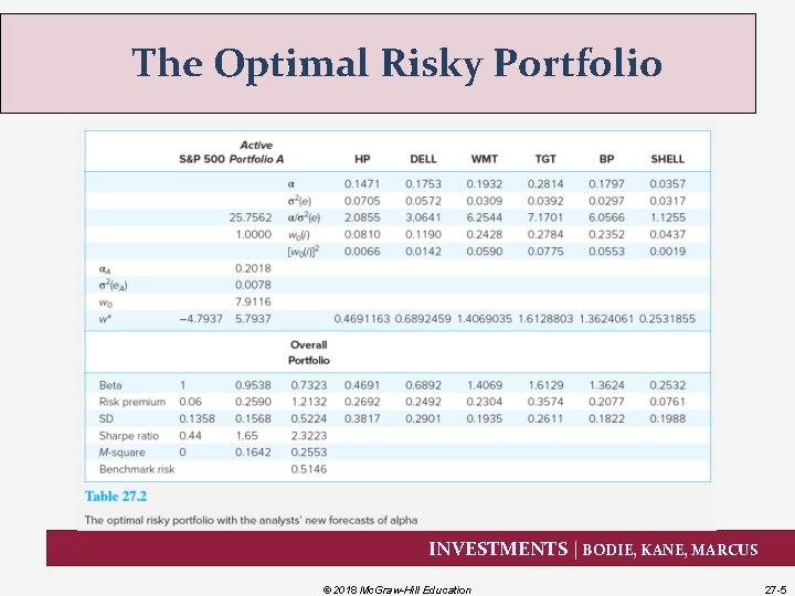
The Optimal Risky Portfolio INVESTMENTS | BODIE, KANE, MARCUS © 2018 Mc. Graw-Hill Education 27 -5

The Optimal Risky Portfolio Results • The Sharpe ratio increases to 2. 32, a huge riskadjusted return advantage • M-square increases to 25. 53% INVESTMENTS | BODIE, KANE, MARCUS © 2018 Mc. Graw-Hill Education 27 -6

Results: Problems • Problems: • The optimal portfolio calls for extreme long/short positions that may not be feasible for a real-world portfolio manager • The portfolio is too risky and most of the risk is nonsystematic risk • A solution: Restrict extreme positions • This results in a lack of diversification INVESTMENTS | BODIE, KANE, MARCUS © 2018 Mc. Graw-Hill Education 27 -7

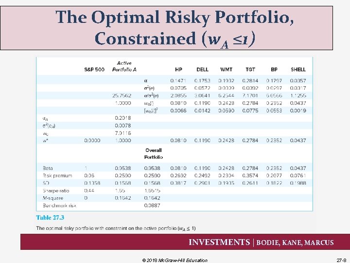
The Optimal Risky Portfolio, Constrained (w. A ≤ 1) INVESTMENTS | BODIE, KANE, MARCUS © 2018 Mc. Graw-Hill Education 27 -8

The Optimal Risky Portfolio, Constrained (w. A ≤ 1) Results • The Sharpe ratio falls from 2. 32 to 1. 65 • M-square is now. 1642 INVESTMENTS | BODIE, KANE, MARCUS © 2018 Mc. Graw-Hill Education 27 -9

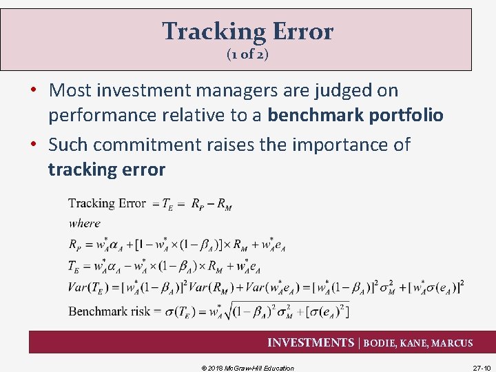
Tracking Error (1 of 2) • Most investment managers are judged on performance relative to a benchmark portfolio • Such commitment raises the importance of tracking error INVESTMENTS | BODIE, KANE, MARCUS © 2018 Mc. Graw-Hill Education 27 -10

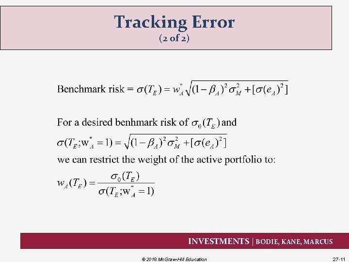
Tracking Error (2 of 2) INVESTMENTS | BODIE, KANE, MARCUS © 2018 Mc. Graw-Hill Education 27 -11

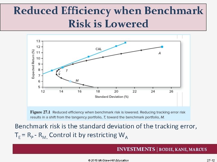
Reduced Efficiency when Benchmark Risk is Lowered Benchmark risk is the standard deviation of the tracking error, TE = RP - RM. Control it by restricting WA INVESTMENTS | BODIE, KANE, MARCUS © 2018 Mc. Graw-Hill Education 27 -12

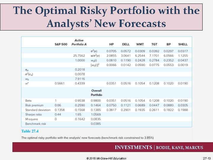
The Optimal Risky Portfolio with the Analysts’ New Forecasts INVESTMENTS | BODIE, KANE, MARCUS © 2018 Mc. Graw-Hill Education 27 -13

The Optimal Risky Portfolio with the Analysts’ New Forecasts Results • The Sharpe ratio falls from 1. 65 to 1. 06 • M-square is now. 0835 INVESTMENTS | BODIE, KANE, MARCUS © 2018 Mc. Graw-Hill Education 27 -14

Adjusting Forecasts for the Precision of Alpha • How accurate is your forecast? • Regress forecast alphas on actual, realized alphas to adjust alpha for the accuracy of the analysts’ previous forecasts INVESTMENTS | BODIE, KANE, MARCUS © 2018 Mc. Graw-Hill Education 27 -15

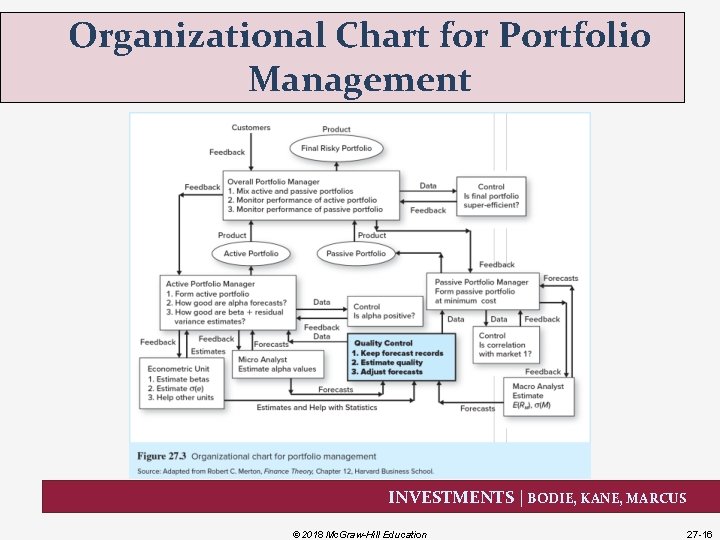
Organizational Chart for Portfolio Management INVESTMENTS | BODIE, KANE, MARCUS © 2018 Mc. Graw-Hill Education 27 -16

The Black-Litterman (BL) Model • The BL model allows portfolio managers to incorporate complex forecasts into the portfolio construction process • Data hails from two sources: history and forecasts, called views • Historical sample is used to estimate covariance matrix and asset allocation to make baseline forecasts • Views represent departure from the baseline, establishing new alpha forecasts and an optimal risky P INVESTMENTS | BODIE, KANE, MARCUS © 2018 Mc. Graw-Hill Education 27 -17

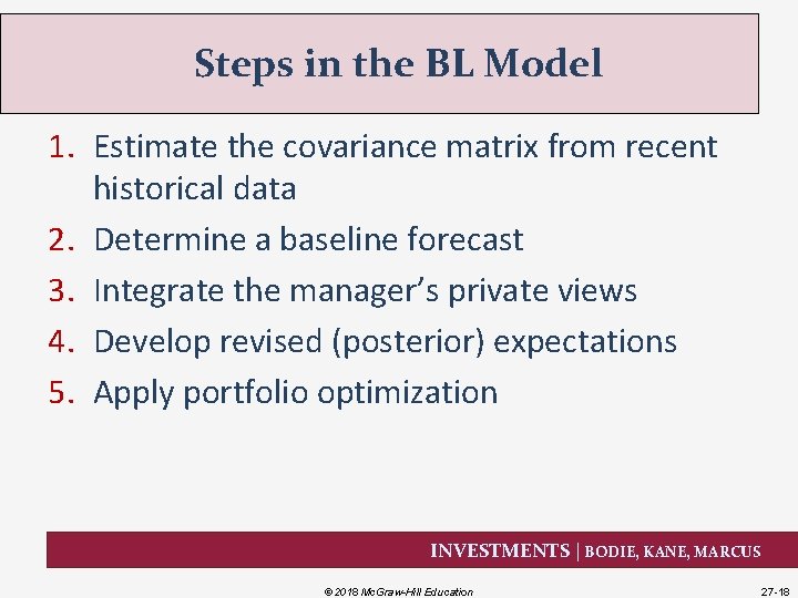
Steps in the BL Model 1. Estimate the covariance matrix from recent historical data 2. Determine a baseline forecast 3. Integrate the manager’s private views 4. Develop revised (posterior) expectations 5. Apply portfolio optimization INVESTMENTS | BODIE, KANE, MARCUS © 2018 Mc. Graw-Hill Education 27 -18

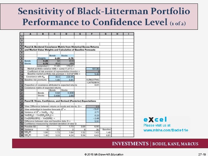
Sensitivity of Black-Litterman Portfolio Performance to Confidence Level (1 of 2) INVESTMENTS | BODIE, KANE, MARCUS © 2018 Mc. Graw-Hill Education 27 -19

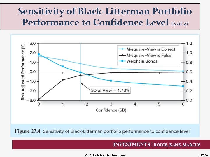
Sensitivity of Black-Litterman Portfolio Performance to Confidence Level (2 of 2) INVESTMENTS | BODIE, KANE, MARCUS © 2018 Mc. Graw-Hill Education 27 -20

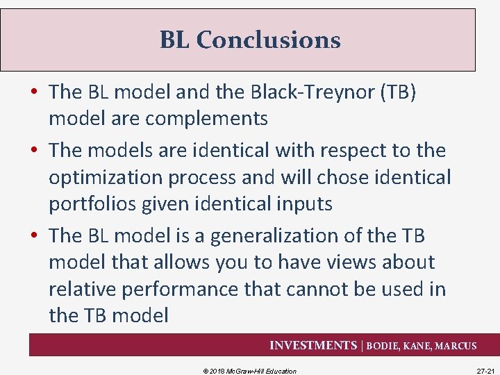
BL Conclusions • The BL model and the Black-Treynor (TB) model are complements • The models are identical with respect to the optimization process and will chose identical portfolios given identical inputs • The BL model is a generalization of the TB model that allows you to have views about relative performance that cannot be used in the TB model INVESTMENTS | BODIE, KANE, MARCUS © 2018 Mc. Graw-Hill Education 27 -21

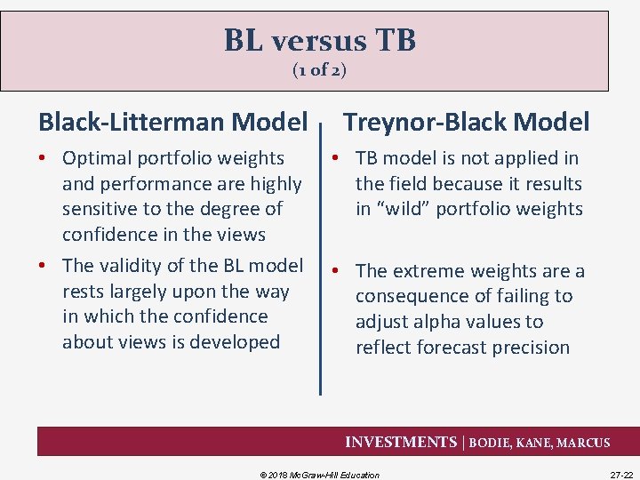
BL versus TB (1 of 2) Black-Litterman Model • Optimal portfolio weights and performance are highly sensitive to the degree of confidence in the views • The validity of the BL model rests largely upon the way in which the confidence about views is developed Treynor-Black Model • TB model is not applied in the field because it results in “wild” portfolio weights • The extreme weights are a consequence of failing to adjust alpha values to reflect forecast precision INVESTMENTS | BODIE, KANE, MARCUS © 2018 Mc. Graw-Hill Education 27 -22

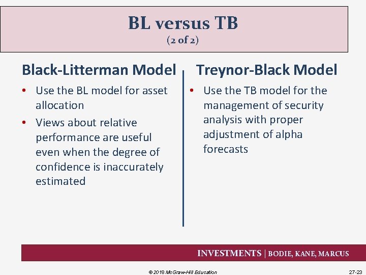
BL versus TB (2 of 2) Black-Litterman Model • Use the BL model for asset allocation • Views about relative performance are useful even when the degree of confidence is inaccurately estimated Treynor-Black Model • Use the TB model for the management of security analysis with proper adjustment of alpha forecasts INVESTMENTS | BODIE, KANE, MARCUS © 2018 Mc. Graw-Hill Education 27 -23

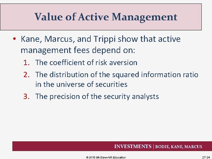
Value of Active Management • Kane, Marcus, and Trippi show that active management fees depend on: 1. The coefficient of risk aversion 2. The distribution of the squared information ratio in the universe of securities 3. The precision of the security analysts INVESTMENTS | BODIE, KANE, MARCUS © 2018 Mc. Graw-Hill Education 27 -24

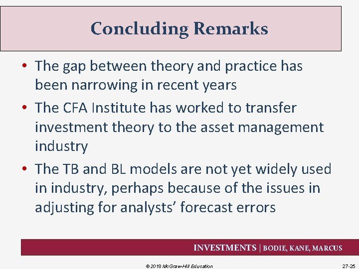
Concluding Remarks • The gap between theory and practice has been narrowing in recent years • The CFA Institute has worked to transfer investment theory to the asset management industry • The TB and BL models are not yet widely used in industry, perhaps because of the issues in adjusting for analysts’ forecast errors INVESTMENTS | BODIE, KANE, MARCUS © 2018 Mc. Graw-Hill Education 27 -25