Chapter Topics Linear Programming Formulation and Applications n

Chapter Topics Linear Programming: Formulation and Applications n Model Formulation n A Maximization Model Example n Graphical Solutions of Linear Programming Models n A Minimization Model Example n Irregular Types of Linear Programming Models n Characteristics of Linear Programming Problems Copyright © 2013 Pearson Education, Inc. Publishing as Prentice Hall 2 -1

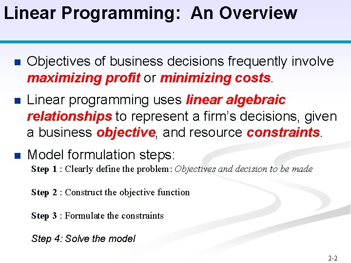
Linear Programming: An Overview n Objectives of business decisions frequently involve maximizing profit or minimizing costs. n Linear programming uses linear algebraic relationships to represent a firm’s decisions, given a business objective, and resource constraints. n Model formulation steps: Step 1 : Clearly define the problem: Objectives and decision to be made Step 2 : Construct the objective function Step 3 : Formulate the constraints Step 4: Solve the model 2 -2

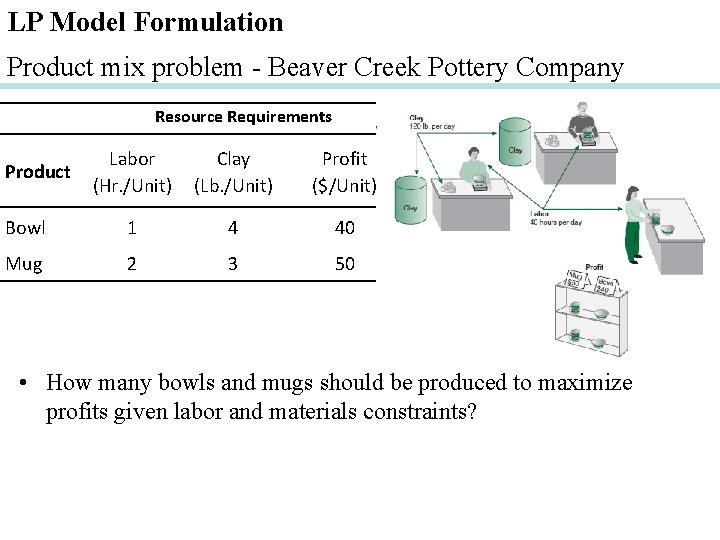
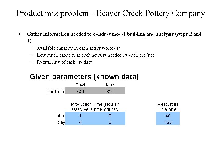
LP Model Formulation Product mix problem - Beaver Creek Pottery Company Resource Requirements Labor (Hr. /Unit) Clay (Lb. /Unit) Profit ($/Unit) Bowl 1 4 40 Mug 2 3 50 Product • How many bowls and mugs should be produced to maximize profits given labor and materials constraints?

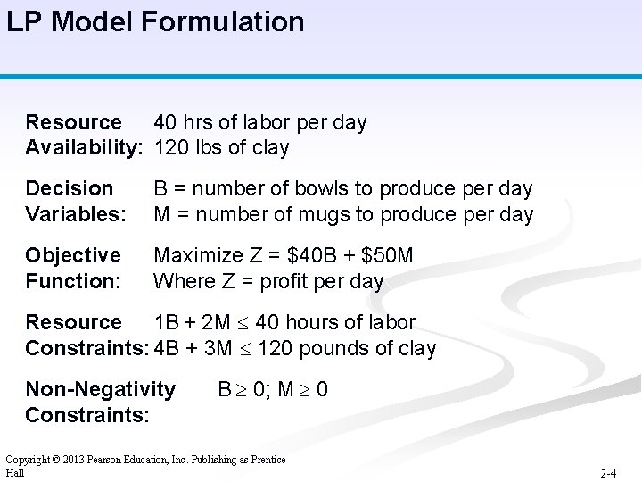
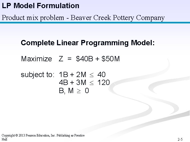
LP Model Formulation Resource 40 hrs of labor per day Availability: 120 lbs of clay Decision B = number of bowls to produce per day Variables: M = number of mugs to produce per day Objective Maximize Z = $40 B + $50 M Function: Where Z = profit per day Resource 1 B + 2 M 40 hours of labor Constraints: 4 B + 3 M 120 pounds of clay Non-Negativity Constraints: B 0; M 0 Copyright © 2013 Pearson Education, Inc. Publishing as Prentice Hall 2 -4

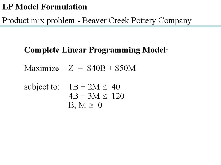
LP Model Formulation Product mix problem - Beaver Creek Pottery Company Complete Linear Programming Model: Maximize Z = $40 B + $50 M subject to: 1 B + 2 M 40 4 B + 3 M 120 B, M 0 Copyright © 2013 Pearson Education, Inc. Publishing as Prentice Hall 2 -5

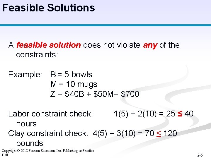
Feasible Solutions A feasible solution does not violate any of the constraints: Example: B = 5 bowls M = 10 mugs Z = $40 B + $50 M= $700 Labor constraint check: 1(5) + 2(10) = 25 ≤ 40 hours Clay constraint check: 4(5) + 3(10) = 70 ≤ 120 pounds Copyright © 2013 Pearson Education, Inc. Publishing as Prentice Hall 2 -6

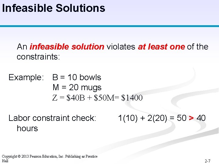
Infeasible Solutions An infeasible solution violates at least one of the constraints: Example: B = 10 bowls M = 20 mugs Z = $40 B + $50 M= $1400 Labor constraint check: hours Copyright © 2013 Pearson Education, Inc. Publishing as Prentice Hall 1(10) + 2(20) = 50 > 40 2 -7

Graphical Solution of LP Models n Graphical solution is limited to linear programming models containing only two decision variables (can be used with three variables but only with great difficulty). n Graphical methods provide visualization of how a solution for a linear programming problem is obtained. Copyright © 2013 Pearson Education, Inc. Publishing as Prentice Hall 2 -8

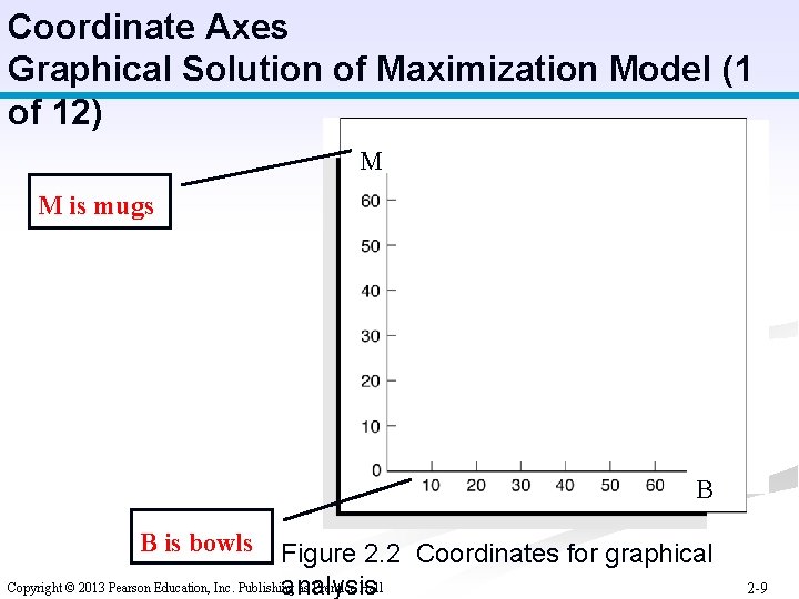
Coordinate Axes Graphical Solution of Maximization Model (1 of 12) M M is mugs B B is bowls Figure 2. 2 Coordinates for graphical Copyright © 2013 Pearson Education, Inc. Publishing as Prentice Hall analysis 2 -9

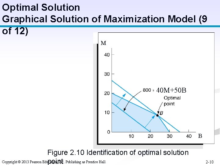
Optimal Solution Graphical Solution of Maximization Model (9 of 12) M 40 M+50 B B Figure 2. 10 Identification of optimal solution Copyright © 2013 Pearson Education, Inc. Publishing as Prentice Hall point 2 -10

Product mix problem - Beaver Creek Pottery Company • Gather information needed to conduct model building and analysis (steps 2 and 3) – Available capacity in each activity/process – How much capacity in each activity needed by each product – Profitability of each product Given parameters (known data) Unit Profit Bowl Mug $40 $50 Production Time (Hours ) Used Per Unit Produced Resources Available labor 1 2 40 clay 4 3 120

LP Model Formulation Product mix problem - Beaver Creek Pottery Company Complete Linear Programming Model: Maximize Z = $40 B + $50 M subject to: 1 B + 2 M 40 4 B + 3 M 120 B, M 0

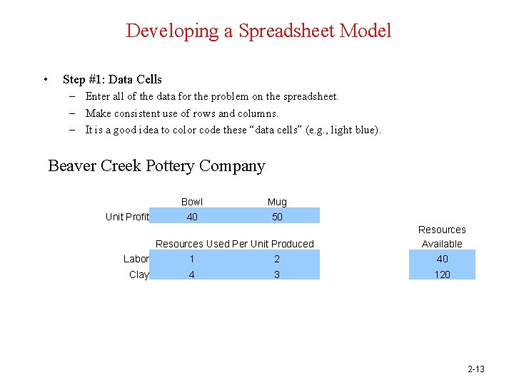
Developing a Spreadsheet Model • Step #1: Data Cells – Enter all of the data for the problem on the spreadsheet. – Make consistent use of rows and columns. – It is a good idea to color code these “data cells” (e. g. , light blue). Beaver Creek Pottery Company Unit Profit Bowl Mug 40 50 Resources Used Per Unit Produced Resources Available Labor 1 2 40 Clay 4 3 120 2 -13

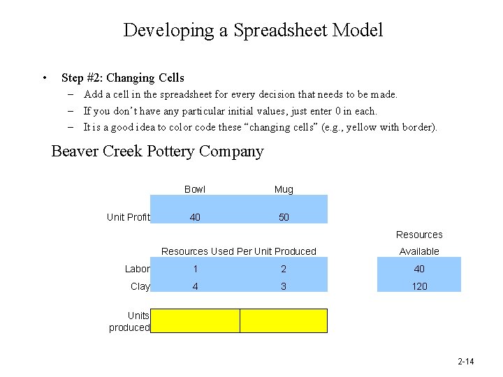
Developing a Spreadsheet Model • Step #2: Changing Cells – Add a cell in the spreadsheet for every decision that needs to be made. – If you don’t have any particular initial values, just enter 0 in each. – It is a good idea to color code these “changing cells” (e. g. , yellow with border). Beaver Creek Pottery Company Unit Profit Bowl Mug 40 50 Resources Used Per Unit Produced Available Labor 1 2 40 Clay 4 3 120 Units produced 2 -14

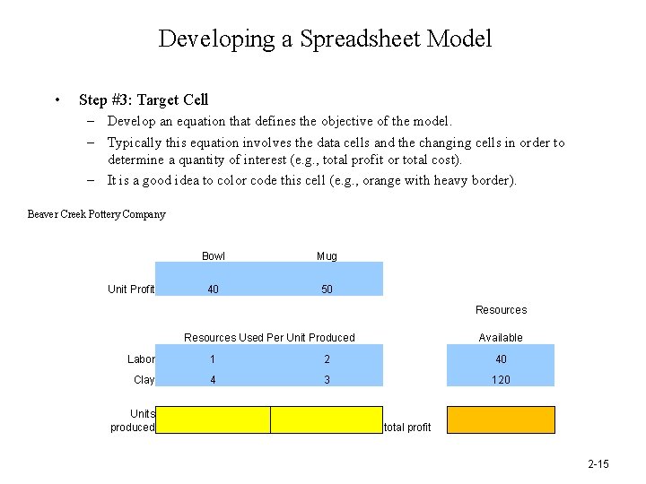
Developing a Spreadsheet Model • Step #3: Target Cell – Develop an equation that defines the objective of the model. – Typically this equation involves the data cells and the changing cells in order to determine a quantity of interest (e. g. , total profit or total cost). – It is a good idea to color code this cell (e. g. , orange with heavy border). Beaver Creek Pottery Company Unit Profit Bowl Mug 40 50 Resources Used Per Unit Produced Available Labor 1 2 40 Clay 4 3 120 Units produced total profit 2 -15

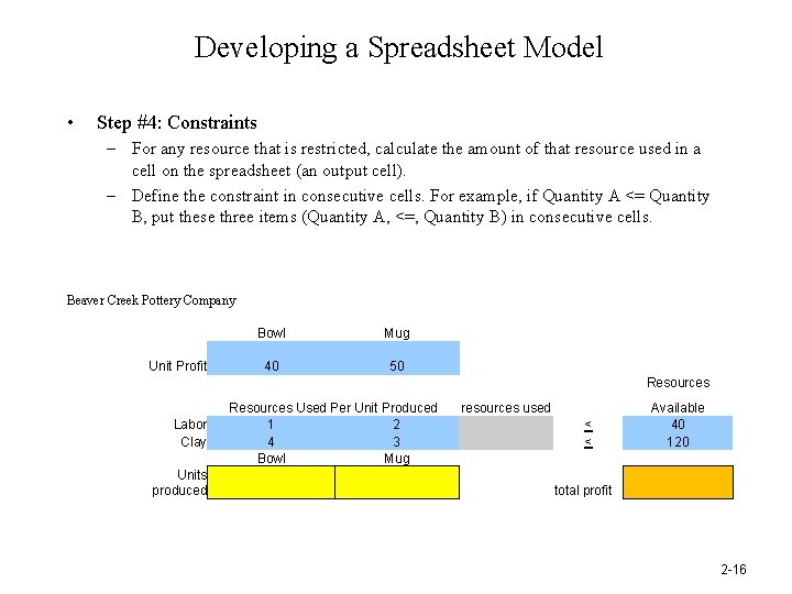
Developing a Spreadsheet Model • Step #4: Constraints – For any resource that is restricted, calculate the amount of that resource used in a cell on the spreadsheet (an output cell). – Define the constraint in consecutive cells. For example, if Quantity A <= Quantity B, put these three items (Quantity A, <=, Quantity B) in consecutive cells. Beaver Creek Pottery Company Unit Profit Bowl Mug 40 50 Resources Labor Clay Units produced Resources Used Per Unit Produced 1 2 4 3 Bowl Mug resources used < < Available 40 120 total profit 2 -16

A Trial Solution Let’s do this problem in Excel…. Pay attention to Model layout and organization Data accuracy Steps in the Solver Addin Max or Min non-negativity option Linear optimization 2 -17

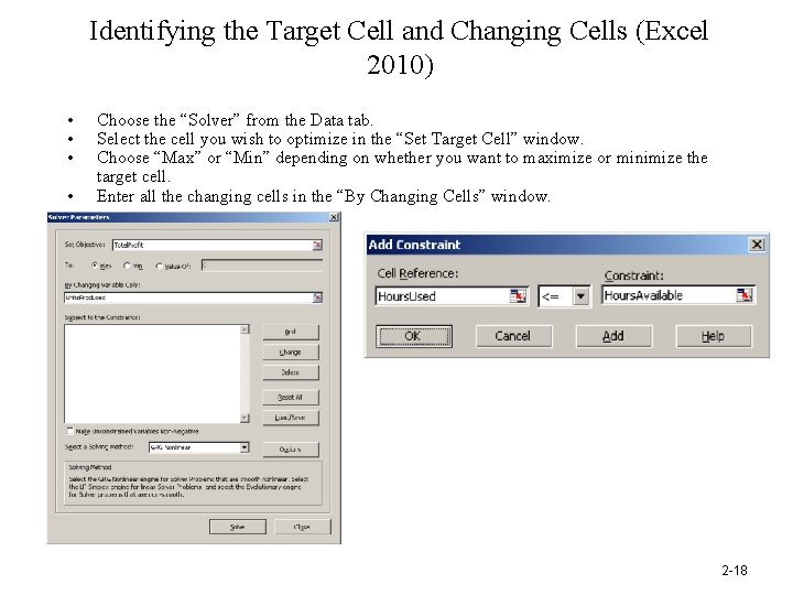
Identifying the Target Cell and Changing Cells (Excel 2010) • • Choose the “Solver” from the Data tab. Select the cell you wish to optimize in the “Set Target Cell” window. Choose “Max” or “Min” depending on whether you want to maximize or minimize the target cell. Enter all the changing cells in the “By Changing Cells” window. 2 -18

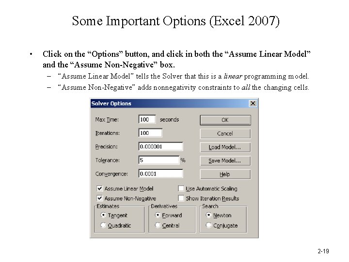
Some Important Options (Excel 2007) • Click on the “Options” button, and click in both the “Assume Linear Model” and the “Assume Non-Negative” box. – “Assume Linear Model” tells the Solver that this is a linear programming model. – “Assume Non-Negative” adds nonnegativity constraints to all the changing cells. 2 -19

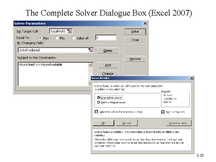
The Complete Solver Dialogue Box (Excel 2007) 2 -20

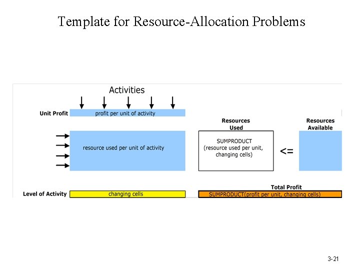
Template for Resource-Allocation Problems 3 -21

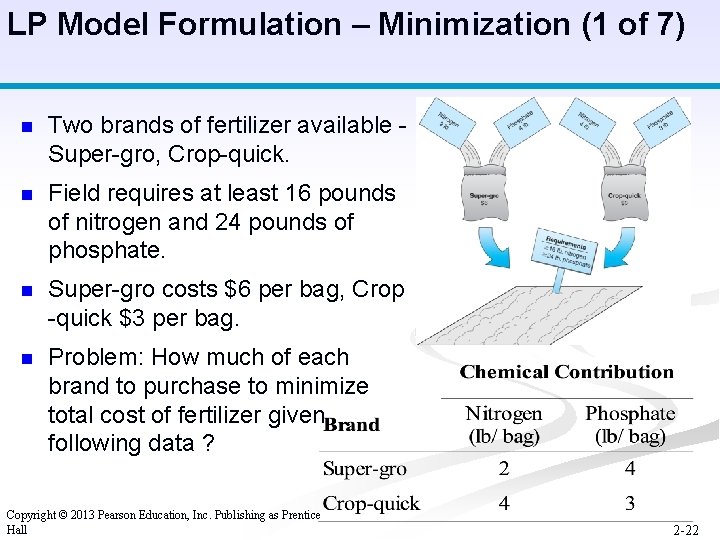
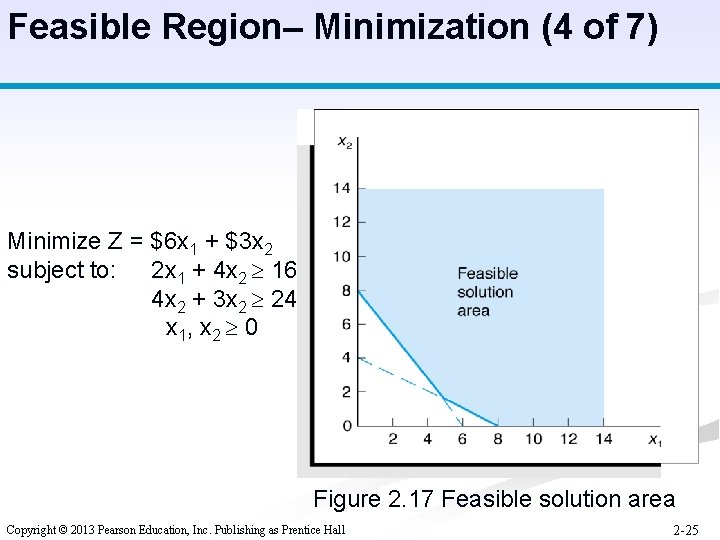
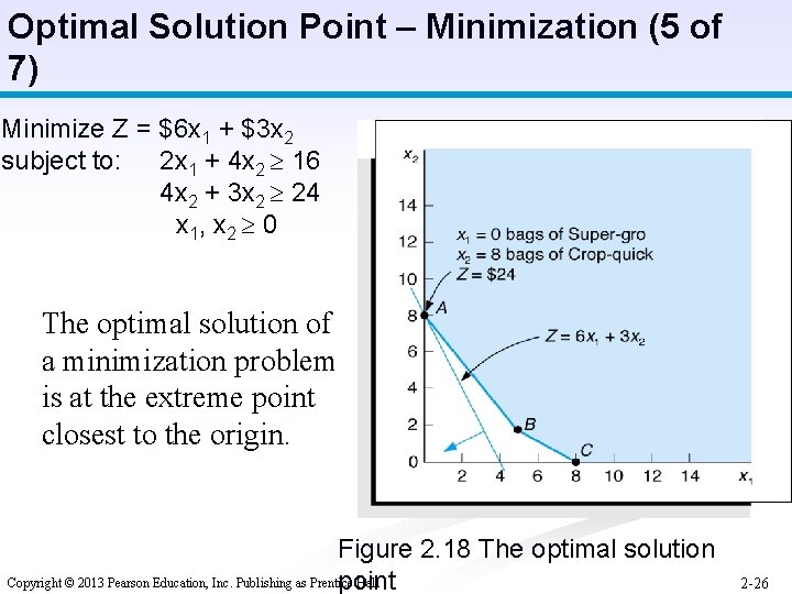
LP Model Formulation – Minimization (1 of 7) n Two brands of fertilizer available - Super-gro, Crop-quick. n Field requires at least 16 pounds of nitrogen and 24 pounds of phosphate. n Super-gro costs $6 per bag, Crop -quick $3 per bag. n Problem: How much of each brand to purchase to minimize total cost of fertilizer given following data ? Copyright © 2013 Pearson Education, Inc. Publishing as Prentice Hall 2 -22

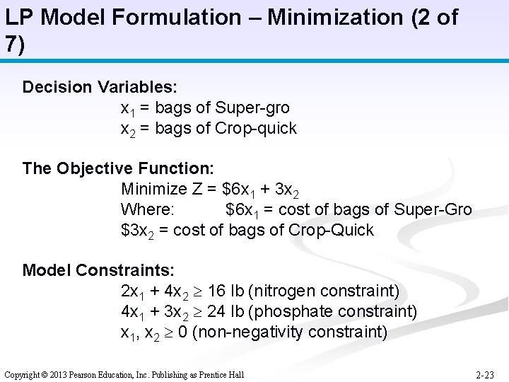
LP Model Formulation – Minimization (2 of 7) Decision Variables: x 1 = bags of Super-gro x 2 = bags of Crop-quick The Objective Function: Minimize Z = $6 x 1 + 3 x 2 Where: $6 x 1 = cost of bags of Super-Gro $3 x 2 = cost of bags of Crop-Quick Model Constraints: 2 x 1 + 4 x 2 16 lb (nitrogen constraint) 4 x 1 + 3 x 2 24 lb (phosphate constraint) x 1, x 2 0 (non-negativity constraint) Copyright © 2013 Pearson Education, Inc. Publishing as Prentice Hall 2 -23

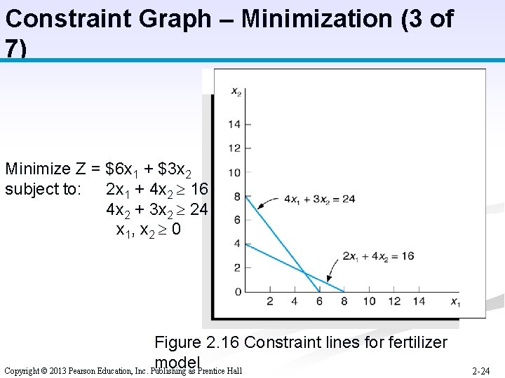
Constraint Graph – Minimization (3 of 7) Minimize Z = $6 x 1 + $3 x 2 subject to: 2 x 1 + 4 x 2 16 4 x 2 + 3 x 2 24 x 1, x 2 0 Figure 2. 16 Constraint lines for fertilizer model Copyright © 2013 Pearson Education, Inc. Publishing as Prentice Hall 2 -24

Feasible Region– Minimization (4 of 7) Minimize Z = $6 x 1 + $3 x 2 subject to: 2 x 1 + 4 x 2 16 4 x 2 + 3 x 2 24 x 1, x 2 0 Figure 2. 17 Feasible solution area Copyright © 2013 Pearson Education, Inc. Publishing as Prentice Hall 2 -25

Optimal Solution Point – Minimization (5 of 7) Minimize Z = $6 x 1 + $3 x 2 subject to: 2 x 1 + 4 x 2 16 4 x 2 + 3 x 2 24 x 1, x 2 0 The optimal solution of a minimization problem is at the extreme point closest to the origin. Figure 2. 18 The optimal solution Copyright © 2013 Pearson Education, Inc. Publishing as Prentice Hall point 2 -26

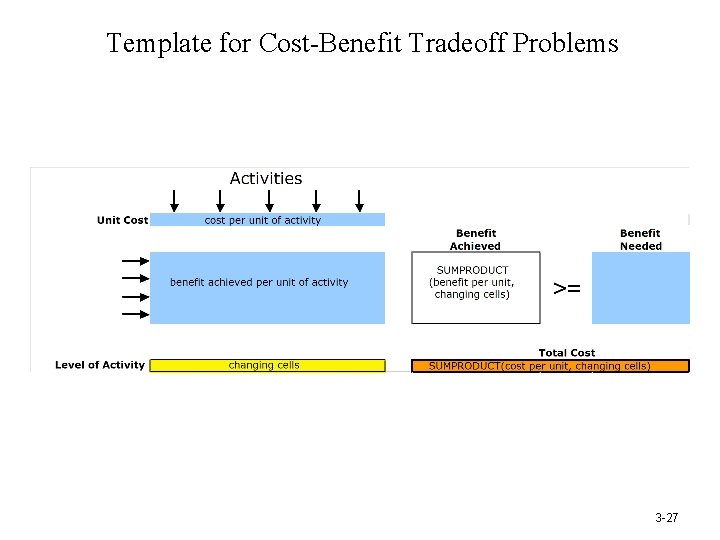
Template for Cost-Benefit Tradeoff Problems 3 -27

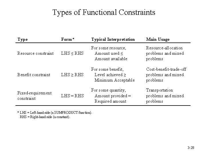
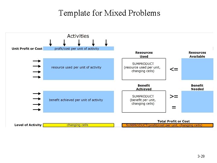
Types of Functional Constraints Type Resource constraint Benefit constraint Fixed-requirement constraint Form* Typical Interpretation Main Usage LHS ≤ RHS For some resource, Amount used ≤ Amount available Resource-allocation problems and mixed problems LHS ≥ RHS For some benefit, Level achieved ≥ Minimum Acceptable Cost-benefit-trade-off problems and mixed problems LHS = RHS For some quantity, Amount provided = Required amount Transportation problems and mixed problems * LHS = Left-hand side (a SUMPRODUCT function). RHS = Right-hand side (a constant). 3 -28

Template for Mixed Problems 3 -29