Chapter Topics Component Factors of the TimeSeries Model

- Slides: 24

Chapter Topics • • Component Factors of the Time-Series Model Smoothing of Data Series Moving Averages o Exponential Smoothing o • Least Square Trend Fitting and Forecasting o • • • Linear, Quadratic and Exponential Models Autoregressive Models Choosing Appropriate Models Monthly or Quarterly Data © 1999 Prentice-Hall, Inc. Chap. 15 - 1

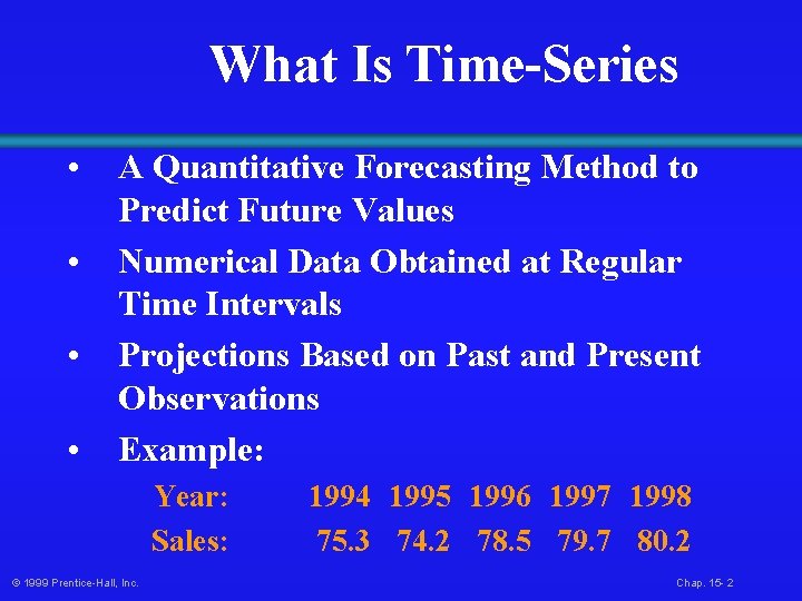
What Is Time-Series • • A Quantitative Forecasting Method to Predict Future Values Numerical Data Obtained at Regular Time Intervals Projections Based on Past and Present Observations Example: Year: Sales: © 1999 Prentice-Hall, Inc. 1994 1995 1996 1997 1998 75. 3 74. 2 78. 5 79. 7 80. 2 Chap. 15 - 2

Time-Series Components Trend Cyclical Time-Series Seasonal © 1999 Prentice-Hall, Inc. Random Chap. 15 - 3

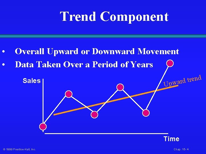
Trend Component • • Overall Upward or Downward Movement Data Taken Over a Period of Years Sales en r t d r a Upw Time © 1999 Prentice-Hall, Inc. Chap. 15 - 4 d

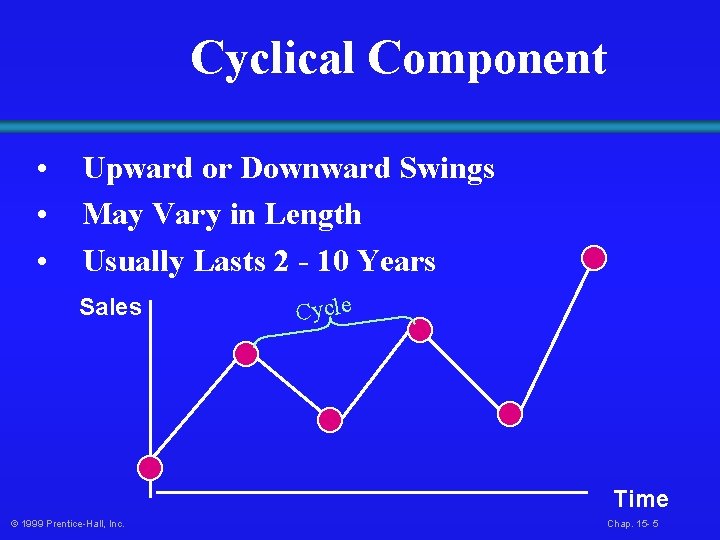
Cyclical Component • • • Upward or Downward Swings May Vary in Length Usually Lasts 2 - 10 Years Sales Cycle Time © 1999 Prentice-Hall, Inc. Chap. 15 - 5

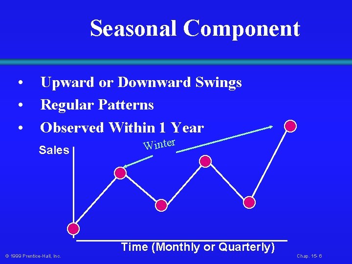
Seasonal Component • • • Upward or Downward Swings Regular Patterns Observed Within 1 Year Sales © 1999 Prentice-Hall, Inc. Winter Time (Monthly or Quarterly) Chap. 15 - 6

Random or Irregular Component • Erratic, Nonsystematic, Random, ‘Residual’ Fluctuations • • Due to Random Variations of o Nature o Accidents Short Duration and Non-repeating © 1999 Prentice-Hall, Inc. Chap. 15 - 7

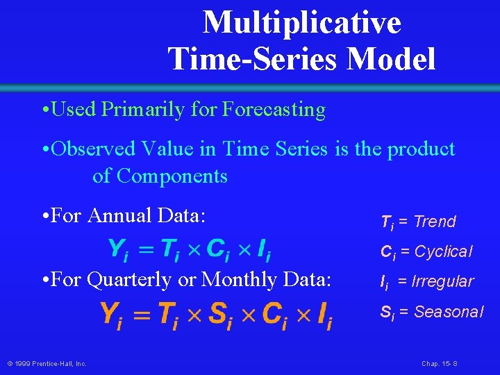
Multiplicative Time-Series Model • Used Primarily for Forecasting • Observed Value in Time Series is the product of Components • For Annual Data: Ti = Trend Ci = Cyclical • For Quarterly or Monthly Data: Ii = Irregular Si = Seasonal © 1999 Prentice-Hall, Inc. Chap. 15 - 8

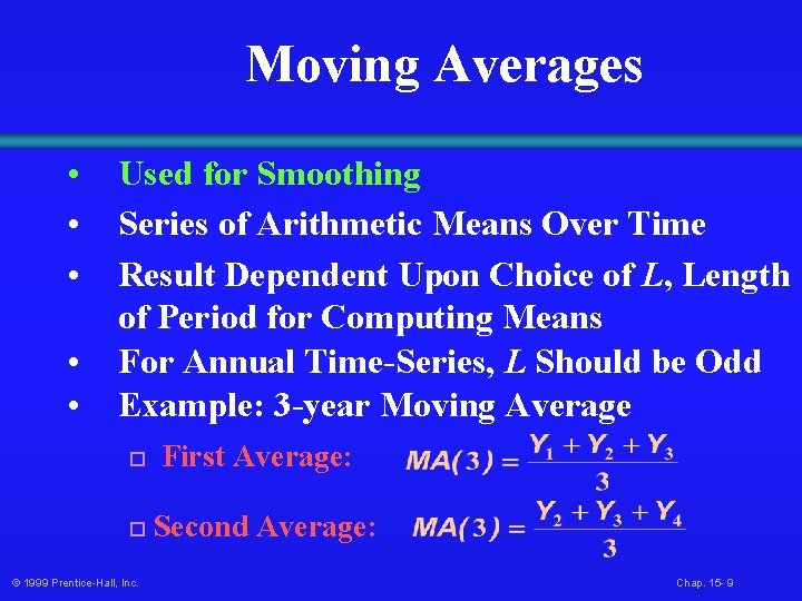
Moving Averages • • • Used for Smoothing Series of Arithmetic Means Over Time Result Dependent Upon Choice of L, Length of Period for Computing Means For Annual Time-Series, L Should be Odd Example: 3 -year Moving Average o o © 1999 Prentice-Hall, Inc. First Average: Second Average: Chap. 15 - 9

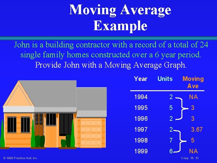
Moving Average Example John is a building contractor with a record of a total of 24 single family homes constructed over a 6 year period. Provide John with a Moving Average Graph. © 1999 Prentice-Hall, Inc. Year Units Moving Ave 1994 2 NA 1995 5 3 1996 2 3 1997 2 3. 67 1998 7 5 1999 6 NA Chap. 15 - 10

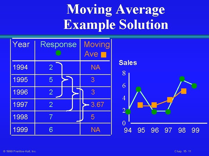
Moving Average Example Solution Year Response Moving Ave 1994 2 NA 1995 5 3 1996 2 3 1997 2 3. 67 1998 7 5 1999 6 NA © 1999 Prentice-Hall, Inc. Sales 8 6 4 2 0 94 95 96 97 98 99 Chap. 15 - 11

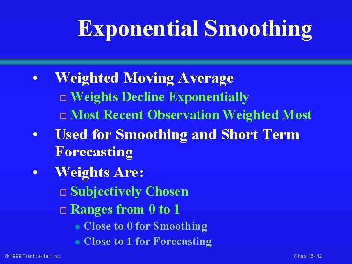
Exponential Smoothing • Weighted Moving Average Weights Decline Exponentially o Most Recent Observation Weighted Most o • • Used for Smoothing and Short Term Forecasting Weights Are: Subjectively Chosen o Ranges from 0 to 1 o Close to 0 for Smoothing l Close to 1 for Forecasting l © 1999 Prentice-Hall, Inc. Chap. 15 - 12

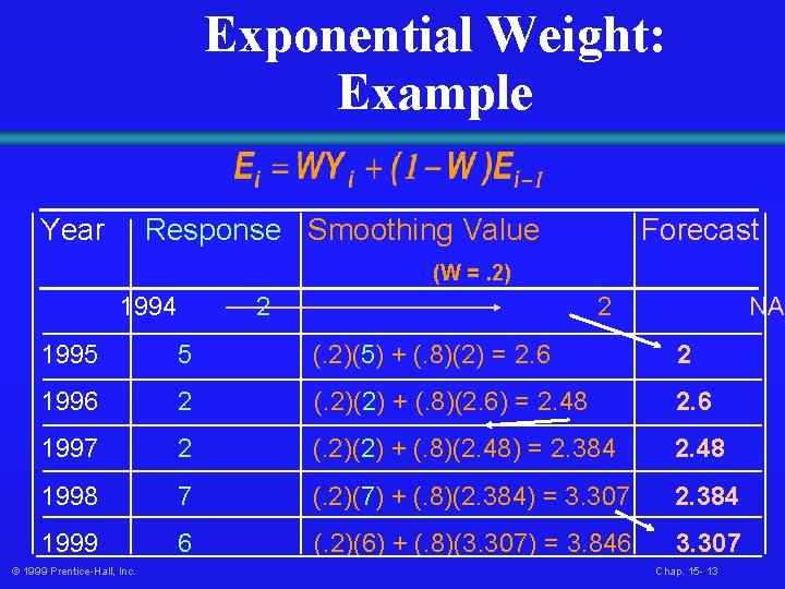
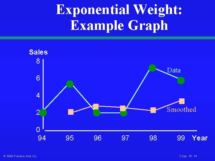
Exponential Weight: Example Year Response Smoothing Value Forecast (W =. 2) 1994 2 2 NA 1995 5 (. 2)(5) + (. 8)(2) = 2. 6 2 1996 2 (. 2)(2) + (. 8)(2. 6) = 2. 48 2. 6 1997 2 (. 2)(2) + (. 8)(2. 48) = 2. 384 2. 48 1998 7 (. 2)(7) + (. 8)(2. 384) = 3. 307 2. 384 1999 6 (. 2)(6) + (. 8)(3. 307) = 3. 846 3. 307 © 1999 Prentice-Hall, Inc. Chap. 15 - 13

Exponential Weight: Example Graph Sales 8 Data 6 4 Smoothed 2 0 94 © 1999 Prentice-Hall, Inc. 95 96 97 98 99 Year Chap. 15 - 14

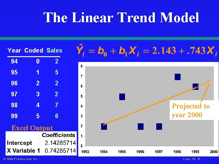
The Linear Trend Model Year Coded Sales 94 0 2 95 1 5 96 2 2 97 3 2 98 4 7 99 5 6 Projected to year 2000 Excel Output © 1999 Prentice-Hall, Inc. Chap. 15 - 15

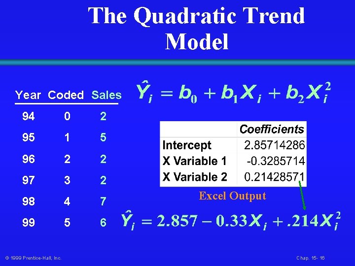
The Quadratic Trend Model Year Coded Sales 94 0 2 95 1 5 96 2 2 97 3 2 98 4 7 99 5 6 © 1999 Prentice-Hall, Inc. Excel Output Chap. 15 - 16

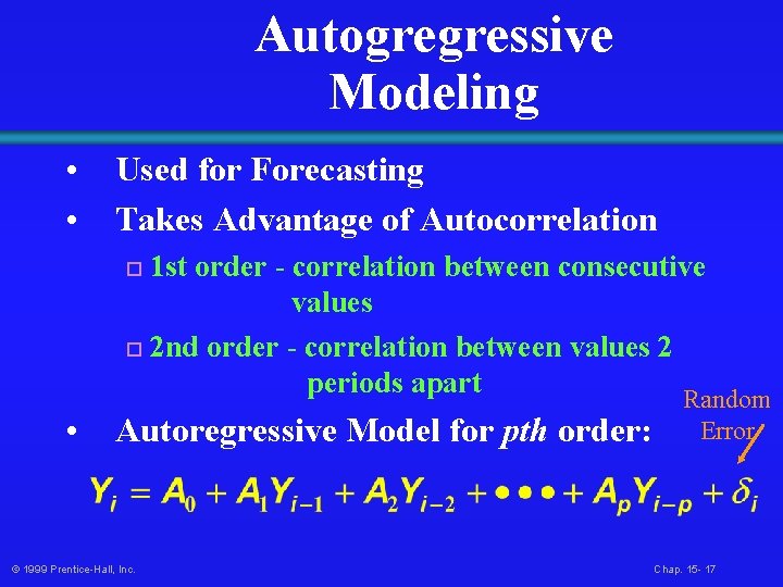
Autogregressive Modeling • • Used for Forecasting Takes Advantage of Autocorrelation 1 st order - correlation between consecutive values o 2 nd order - correlation between values 2 periods apart Random o • Autoregressive Model for pth order: © 1999 Prentice-Hall, Inc. Error Chap. 15 - 17

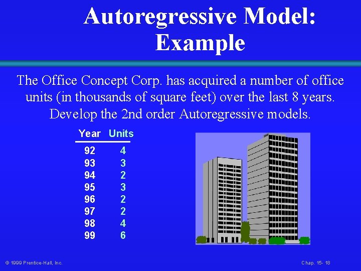
Autoregressive Model: Example The Office Concept Corp. has acquired a number of office units (in thousands of square feet) over the last 8 years. Develop the 2 nd order Autoregressive models. Year Units 92 93 94 95 96 97 98 99 © 1999 Prentice-Hall, Inc. 4 3 2 2 4 6 Chap. 15 - 18

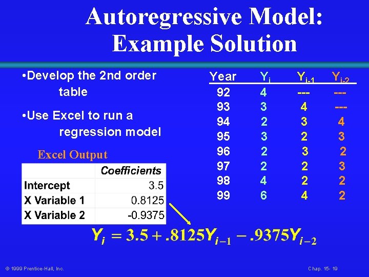
Autoregressive Model: Example Solution • Develop the 2 nd order table • Use Excel to run a regression model Excel Output © 1999 Prentice-Hall, Inc. Year 92 93 94 95 96 97 98 99 Yi 4 3 2 2 4 6 Yi-1 --4 3 2 2 4 Yi-2 ----4 3 2 2 Chap. 15 - 19

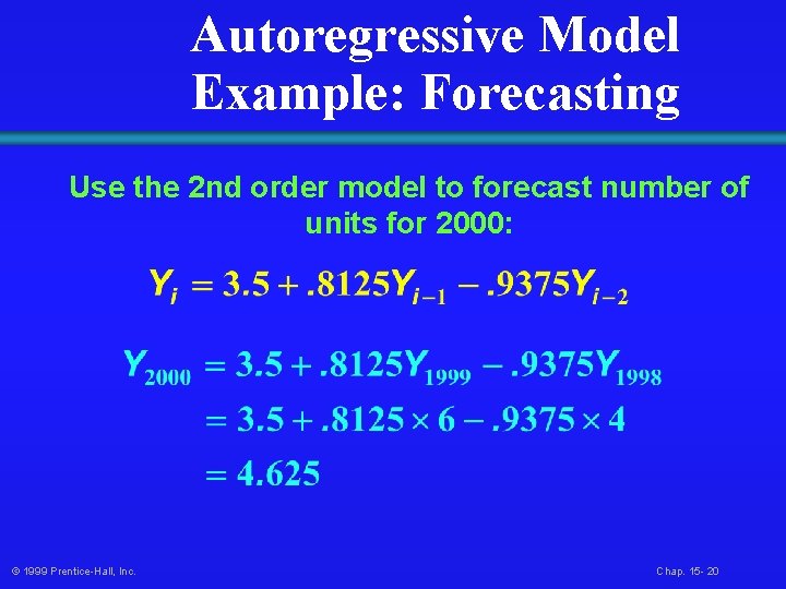
Autoregressive Model Example: Forecasting Use the 2 nd order model to forecast number of units for 2000: © 1999 Prentice-Hall, Inc. Chap. 15 - 20

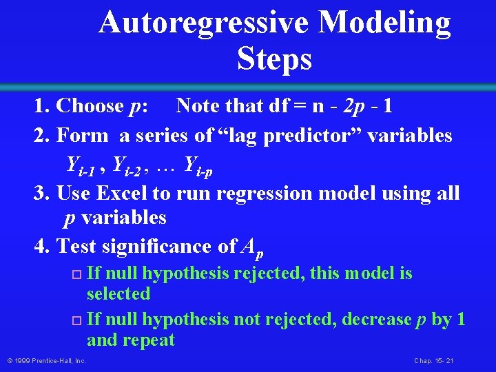
Autoregressive Modeling Steps 1. Choose p: Note that df = n - 2 p - 1 2. Form a series of “lag predictor” variables Yi-1 , Yi-2 , … Yi-p 3. Use Excel to run regression model using all p variables 4. Test significance of Ap If null hypothesis rejected, this model is selected o If null hypothesis not rejected, decrease p by 1 and repeat o © 1999 Prentice-Hall, Inc. Chap. 15 - 21

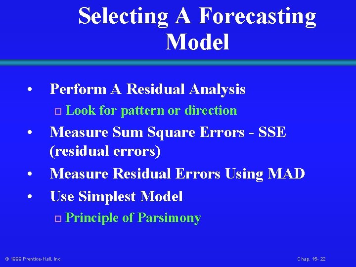
Selecting A Forecasting Model • Perform A Residual Analysis o • • • Look for pattern or direction Measure Sum Square Errors - SSE (residual errors) Measure Residual Errors Using MAD Use Simplest Model o © 1999 Prentice-Hall, Inc. Principle of Parsimony Chap. 15 - 22

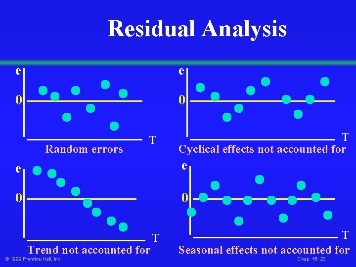
Residual Analysis e e 0 0 Random errors T T Cyclical effects not accounted for e e 0 0 Trend not accounted for © 1999 Prentice-Hall, Inc. T T Seasonal effects not accounted for Chap. 15 - 23

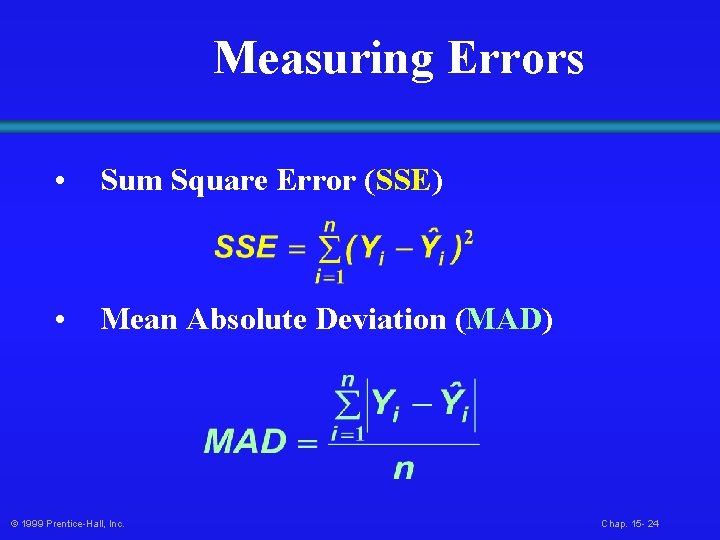
Measuring Errors • Sum Square Error (SSE) • Mean Absolute Deviation (MAD) © 1999 Prentice-Hall, Inc. Chap. 15 - 24