Chapter Three Plotting 2152022 Matlab Diyar Rasoolsu edu

Chapter Three: Plotting 2/15/2022 Matlab Diyar. Rasool@su. edu. krd 1

3. Basic Plots v MATLAB has an excellent set of graphic tools. v. Plotting a given data set or the results of computation is possible with very few commands. v. Being able to plot mathematical functions and data freely is the one most important step, and this section is written to assist you to do just that. 2/15/2022 Matlab 2

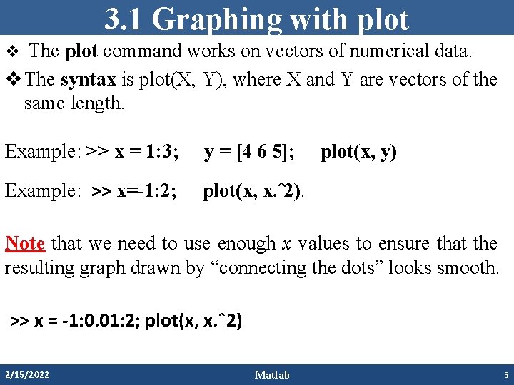
3. 1 Graphing with plot v The plot command works on vectors of numerical data. v The syntax is plot(X, Y), where X and Y are vectors of the same length. Example: >> x = 1: 3; y = [4 6 5]; Example: >> x=-1: 2; plot(x, x. ˆ2). plot(x, y) Note that we need to use enough x values to ensure that the resulting graph drawn by “connecting the dots” looks smooth. >> x = -1: 0. 01: 2; plot(x, x. ˆ2) 2/15/2022 Matlab 3

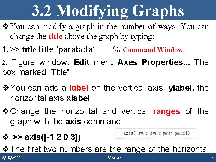
3. 2 Modifying Graphs v You can modify a graph in the number of ways. You can change the title above the graph by typing: 1. >> title 'parabola’ % Command Window. 2. Figure window: Edit menu-Axes Properties. . . The box marked “Title” v You can add a label on the vertical axis: ylabel, the horizontal axis xlabel. v Change the horizontal and vertical ranges of the graph with the axis command. v >> axis([-1 2 0 3]) v The first two numbers are the range of the horizontal 2/15/2022 Matlab axis. 4

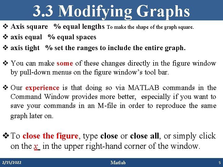
3. 3 Modifying Graphs v Axis square % equal lengths To make the shape of the graph square. v axis equal % equal spaces v axis tight % set the ranges to include the entire graph. v You can make some of these changes directly in the figure window by pull-down menus on the figure window’s tool bar. v Our experience is that doing so via MATLAB commands in the Command Window provides more better, especially if you want to save your commands in an M-file in order to reproduce the same graph later on. v To close the figure, type close or close all, or simply click on the x in the upper right-hand corner of the window. 2/15/2022 Matlab 5

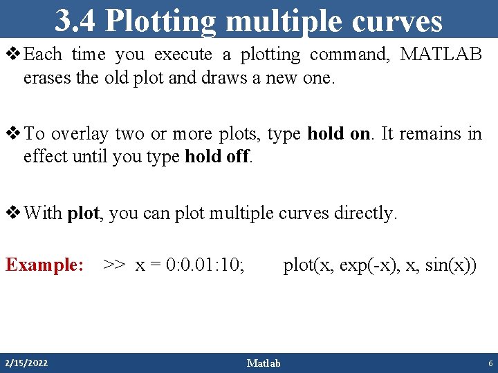
3. 4 Plotting multiple curves v Each time you execute a plotting command, MATLAB erases the old plot and draws a new one. v To overlay two or more plots, type hold on. It remains in effect until you type hold off. v With plot, you can plot multiple curves directly. Example: 2/15/2022 >> x = 0: 0. 01: 10; plot(x, exp(-x), x, sin(x)) Matlab 6

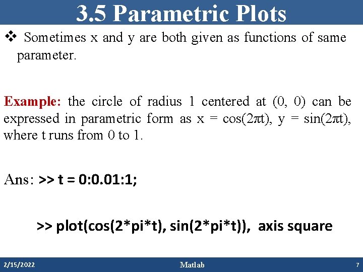
3. 5 Parametric Plots v Sometimes x and y are both given as functions of same parameter. Example: the circle of radius 1 centered at (0, 0) can be expressed in parametric form as x = cos(2πt), y = sin(2πt), where t runs from 0 to 1. Ans: >> t = 0: 0. 01: 1; >> plot(cos(2*pi*t), sin(2*pi*t)), axis square 2/15/2022 Matlab 7

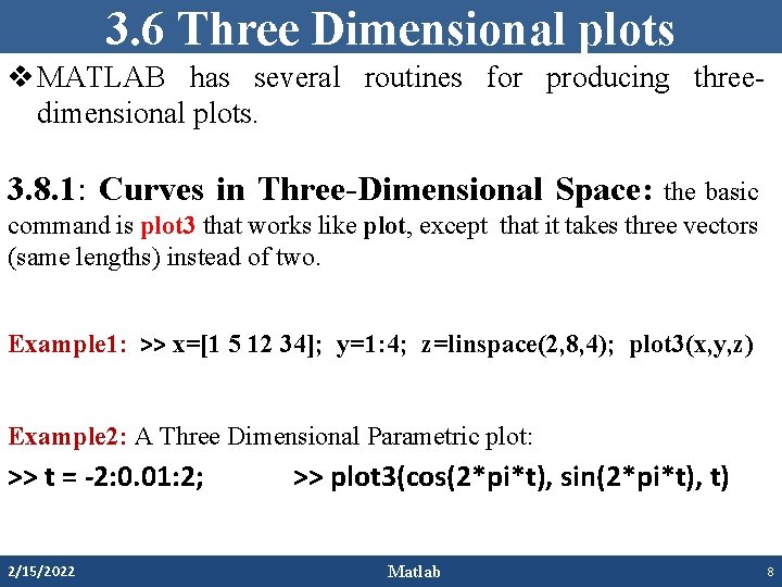
3. 6 Three Dimensional plots v MATLAB has several routines for producing threedimensional plots. 3. 8. 1: Curves in Three-Dimensional Space: the basic command is plot 3 that works like plot, except that it takes three vectors (same lengths) instead of two. Example 1: >> x=[1 5 12 34]; y=1: 4; z=linspace(2, 8, 4); plot 3(x, y, z) Example 2: A Three Dimensional Parametric plot: >> t = -2: 0. 01: 2; 2/15/2022 >> plot 3(cos(2*pi*t), sin(2*pi*t), t) Matlab 8

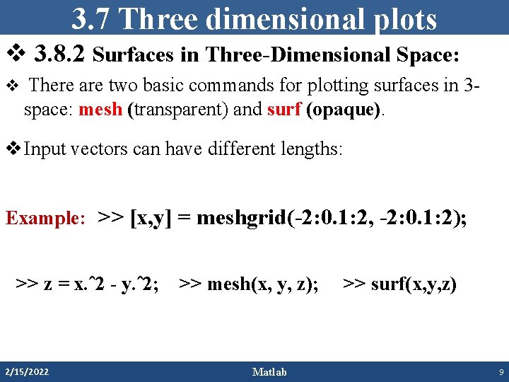
3. 7 Three dimensional plots v 3. 8. 2 Surfaces in Three-Dimensional Space: v There are two basic commands for plotting surfaces in 3 - space: mesh (transparent) and surf (opaque). v Input vectors can have different lengths: Example: >> [x, y] = meshgrid(-2: 0. 1: 2, -2: 0. 1: 2); >> z = x. ˆ2 - y. ˆ2; 2/15/2022 >> mesh(x, y, z); Matlab >> surf(x, y, z) 9

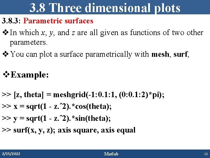
3. 8 Three dimensional plots 3. 8. 3: Parametric surfaces v In which x, y, and z are all given as functions of two other parameters. v You can plot a surface parametrically with mesh, surf, v. Example: >> [z, theta] = meshgrid(-1: 0. 1: 1, (0: 0. 1: 2)*pi); >> x = sqrt(1 - z. ˆ2). *cos(theta); >> y = sqrt(1 - z. ˆ2). *sin(theta); >> surf(x, y, z); axis square, axis equal 2/15/2022 Matlab 10

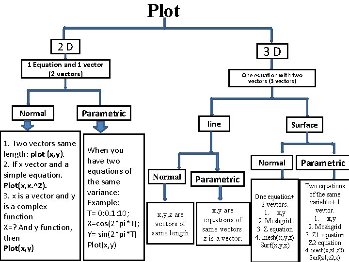
Plot 2 D 3 D 1 Equation and 1 vector (2 vectors) Normal 1. Two vectors same length: plot (x, y). 2. If x vector and a simple equation. Plot(x, x. ^2). 3. x is a vector and y is a complex function X=? And y function, then Plot(x, y) One equation with two vectors (3 vectors) Parametric When you have two equations of the same variance: Example: T= 0: 0. 1: 10; X=cos(2*pi*T); Y= sin(2*pi*T) Plot(x, y) line Surface Normal x, y, z are vectors of same length Parametric x, y are equations of same vectors. z is a vector. One equation+ 2 vevtors. 1. x, y 2. Meshgrid 3. Z equation 4. mesh(x, y, z) Surf(x, y, z) Parametric Two equations of the same variable+ 1 vevtor. 1. x, y 2. Meshgrid 3. Z 1 equation Z 2 equation 4. mesh(x, z 1, z 2) Surf(z 1, z 2, x)

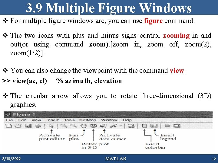
3. 9 Multiple Figure Windows v For multiple figure windows are, you can use figure command. v The two icons with plus and minus signs control zooming in and out(or using command zoom). [zoom in, zoom off, zoom(2), zoom(1/2)]. v You can also change the viewpoint with the command view. >> view(az, el) % azimuth, elevation v The circular arrow allows you to rotate three-dimensional (3 D) graphics. 2/15/2022 MATLAB 12

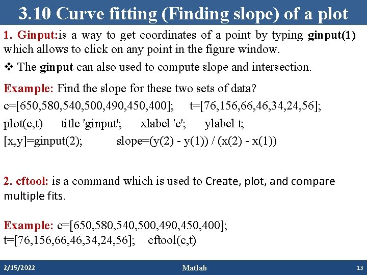
3. 10 Curve fitting (Finding slope) of a plot 1. Ginput: is a way to get coordinates of a point by typing ginput(1) which allows to click on any point in the figure window. v The ginput can also used to compute slope and intersection. Example: Find the slope for these two sets of data? c=[650, 580, 540, 500, 490, 450, 400]; t=[76, 156, 66, 46, 34, 24, 56]; plot(c, t) title 'ginput'; xlabel 'c'; ylabel t; [x, y]=ginput(2); slope=(y(2) - y(1)) / (x(2) - x(1)) 2. cftool: is a command which is used to Create, plot, and compare multiple fits. Example: c=[650, 580, 540, 500, 490, 450, 400]; t=[76, 156, 66, 46, 34, 24, 56]; cftool(c, t) 2/15/2022 Matlab 13

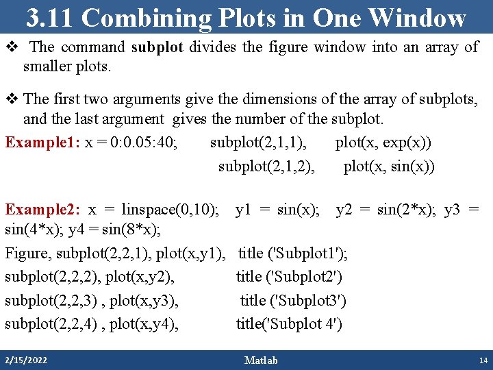
3. 11 Combining Plots in One Window v The command subplot divides the figure window into an array of smaller plots. v The first two arguments give the dimensions of the array of subplots, and the last argument gives the number of the subplot. Example 1: x = 0: 0. 05: 40; subplot(2, 1, 1), plot(x, exp(x)) subplot(2, 1, 2), plot(x, sin(x)) Example 2: x = linspace(0, 10); sin(4*x); y 4 = sin(8*x); Figure, subplot(2, 2, 1), plot(x, y 1), subplot(2, 2, 2), plot(x, y 2), subplot(2, 2, 3) , plot(x, y 3), subplot(2, 2, 4) , plot(x, y 4), 2/15/2022 y 1 = sin(x); y 2 = sin(2*x); y 3 = title ('Subplot 1'); title ('Subplot 2') title ('Subplot 3') title('Subplot 4') Matlab 14

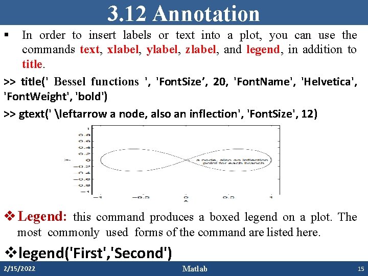
3. 12 Annotation § In order to insert labels or text into a plot, you can use the commands text, xlabel, ylabel, zlabel, and legend, in addition to title. >> title(' Bessel functions ', 'Font. Size’, 20, 'Font. Name', 'Helvetica', 'Font. Weight', 'bold') >> gtext(' leftarrow a node, also an inflection', 'Font. Size', 12) v Legend: this command produces a boxed legend on a plot. The most commonly used forms of the command are listed here. vlegend('First', 'Second') 2/15/2022 Matlab 15

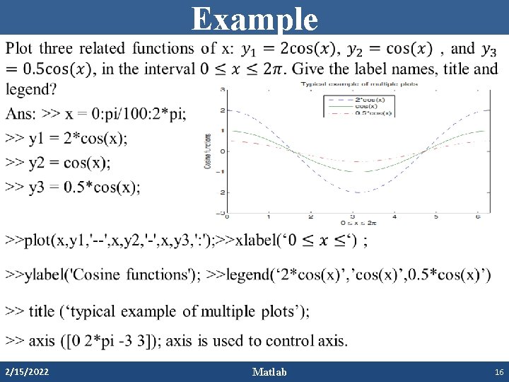
Example • 2/15/2022 Matlab 16

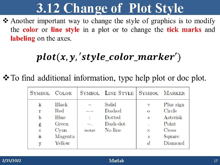
3. 12 Change of Plot Style • 2/15/2022 Matlab 17

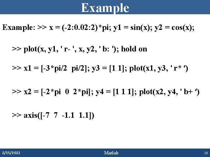
Example: >> x = (-2: 0. 02: 2)*pi; y 1 = sin(x); y 2 = cos(x); >> plot(x, y 1, ' r- ', x, y 2, ' b: '); hold on >> x 1 = [-3*pi/2]; y 3 = [1 1]; plot(x 1, y 3, ' r* ‘) >> x 2 = [-2*pi 0 2*pi]; y 4 = [1 1 1]; plot(x 2, y 4, ' b+ ‘) >> axis([-7 7 -1. 1]) 2/15/2022 Matlab 18

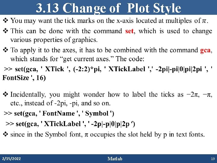
3. 13 Change of Plot Style • 2/15/2022 Matlab 19

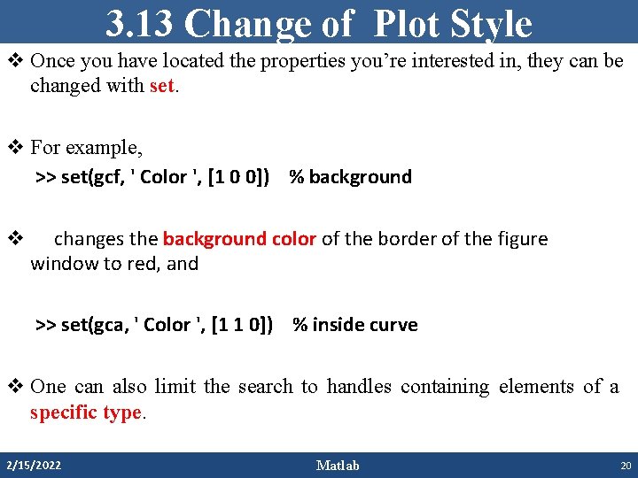
3. 13 Change of Plot Style v Once you have located the properties you’re interested in, they can be changed with set. v For example, >> set(gcf, ' Color ', [1 0 0]) % background v changes the background color of the border of the figure window to red, and >> set(gca, ' Color ', [1 1 0]) % inside curve v One can also limit the search to handles containing elements of a specific type. 2/15/2022 Matlab 20

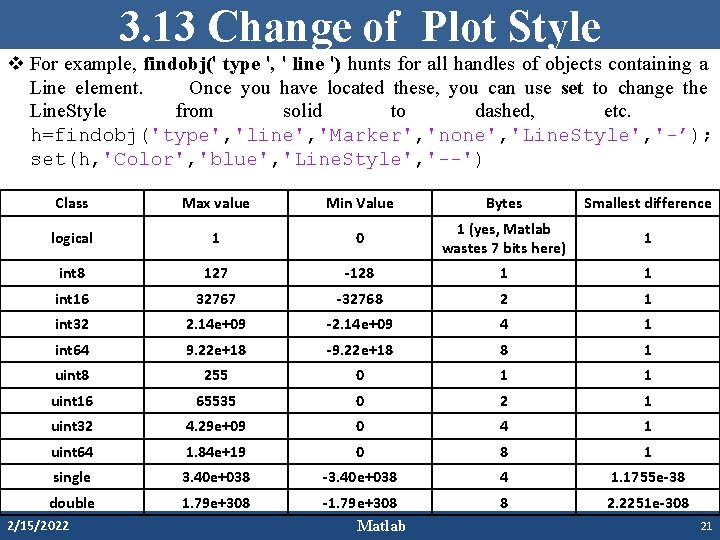
3. 13 Change of Plot Style v For example, findobj(' type ', ' line ') hunts for all handles of objects containing a Line element. Once you have located these, you can use set to change the Line. Style from solid to dashed, etc. h=findobj('type', 'line', 'Marker', 'none', 'Line. Style', '-’); set(h, 'Color', 'blue', 'Line. Style', '--') Class Max value Min Value Bytes Smallest difference logical 1 0 1 (yes, Matlab wastes 7 bits here) 1 int 8 127 -128 1 1 int 16 32767 -32768 2 1 int 32 2. 14 e+09 -2. 14 e+09 4 1 int 64 9. 22 e+18 -9. 22 e+18 8 1 uint 8 255 0 1 1 uint 16 65535 0 2 1 uint 32 4. 29 e+09 0 4 1 uint 64 1. 84 e+19 0 8 1 single 3. 40 e+038 -3. 40 e+038 4 1. 1755 e-38 double 1. 79 e+308 -1. 79 e+308 Matlab 8 2. 2251 e-308 2/15/2022 21