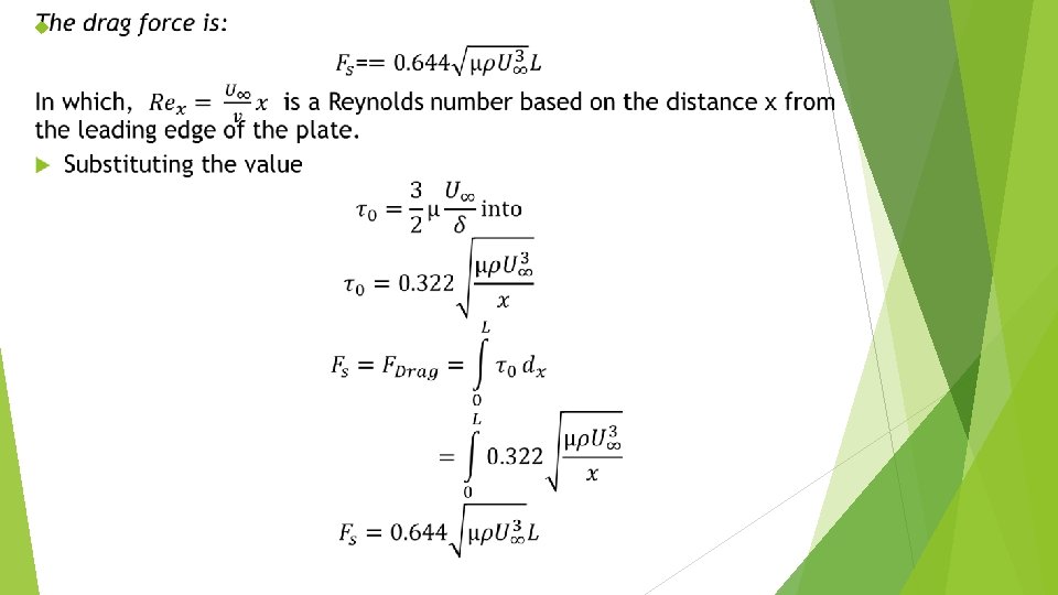
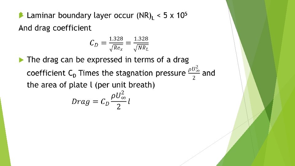
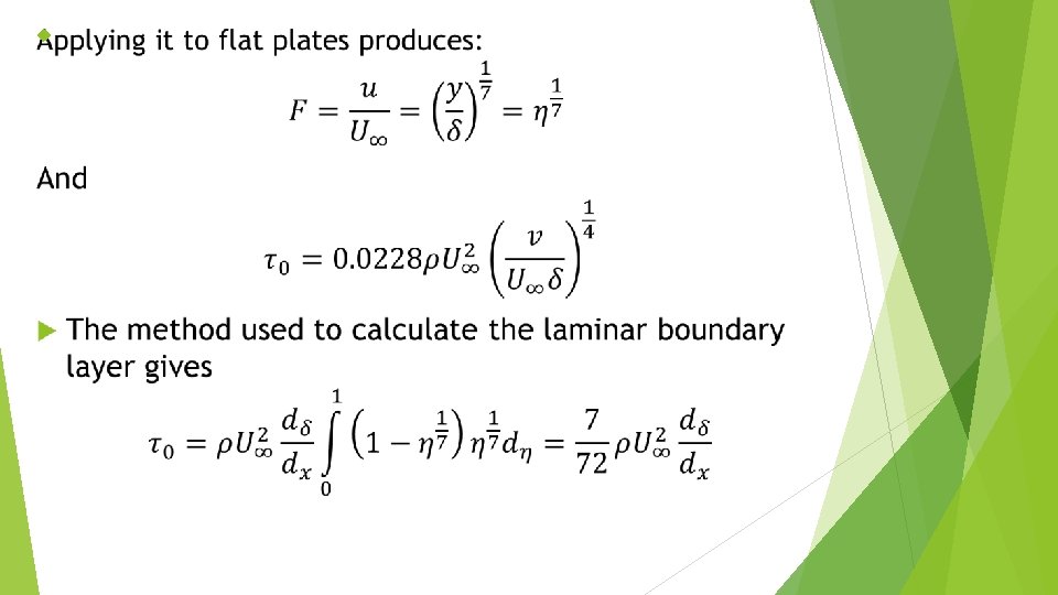
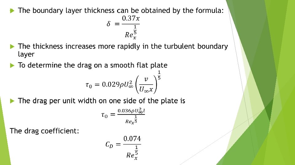
Chapter Three Boundary Layer Theory When real fluid

Chapter Three Boundary Layer Theory When real fluid flows pass a solid boundary the layer that is in contact with the boundary can’t slip away from it and will have same velocity as that of the boundary, this condition is known as “no slip condition” If a fluid boundary is moving, the fluid adhering to it will have the same velocity as that of the boundary. If the boundary is stationary, the fluid velocity at the boundary surface will be zero. Thus at the boundary surface the layer of the fluid undergoes retardation to flow Retardation goes further to adjacent layers A small region in the immediate vicinity of the boundary surface in which the velocity of flowing fluid increases gradually from zero at the boundary surface to the velocity of the main stream. This region is known as boundary layer.

Flow is considered to have two regions: 1. Close to the boundary layer : due to larger velocity gradient appreciable viscous forces are produced. In this region the effect of viscosity is mostly confined, 2. Outside the boundary layer zone: in which the viscous forces are negligible and hence the flow may be treated as non-viscous or in viscid. Prendtl’s boundary layer theory In 1904 prendtl developed the concept of the boundary layer. He provided an important link between ideal- fluid flow and real-fluid flow. For fluids having high Reynold’s number, no matter how small the viscous forces might be in the main flow they become large next to the solid surface, In this region he called a boundary layer the velocity changes from large value at the edge of the boundary layer to zero at the surface of the solid.

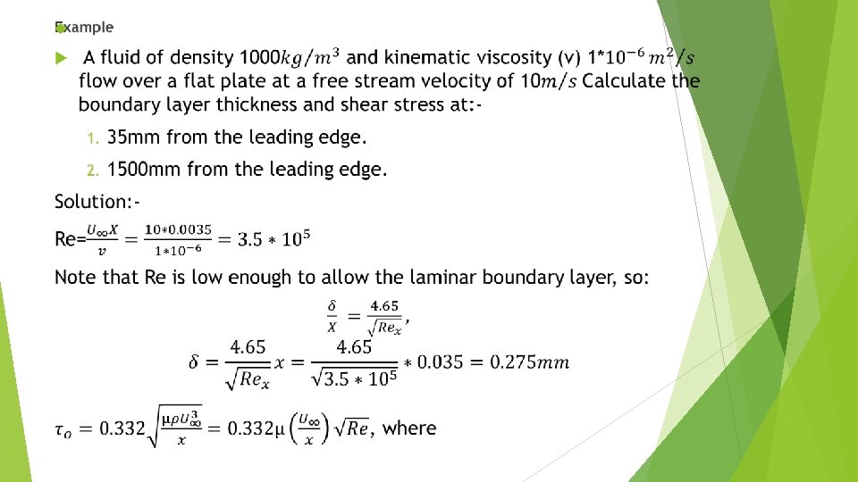
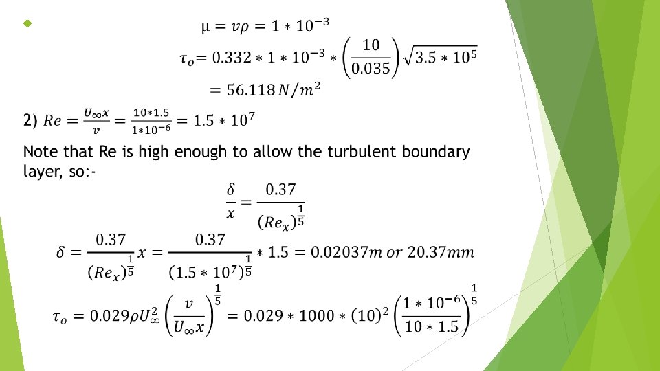
3. 1 Description of the Boundary Layer Consider a flow bounded on one side only the flow just upstream of the plate) has a uniform velocity U∞. As the flow comes into contact with the plate, the layer of fluid immediately adjacent to the plate decelerates (due to viscous friction) and comes to rest.

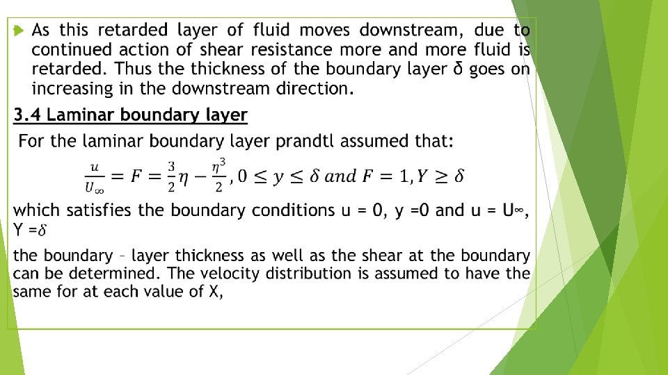
3. 3 Boundary layer along a long thin plate At the leading edge of the plate thickness of the boundary layer is zero, but on downstream, for the fluid in contact with the boundary the velocity of flow is reduced to zero.

Turbulent boundary layer

Separation of boundary layer On a long flat plate the boundary layer continues to grow in the downstream direction, regardless of the length of the plate, when the pressure gradient remains zero, with the pressure decreasing in the downstream direction, the boundary layer tends to be reducing in thickness. For adverse pressure gradients, for that pressure increasing in the downstream direction, the boundary layer thickness rapidly increases. The adverse gradient and the boundary shear decrease the momentum in the boundary layer, and if both act over a sufficient distance, they cause the boundary layer to come to rest. This phenomenon is called separation of the boundary layer.

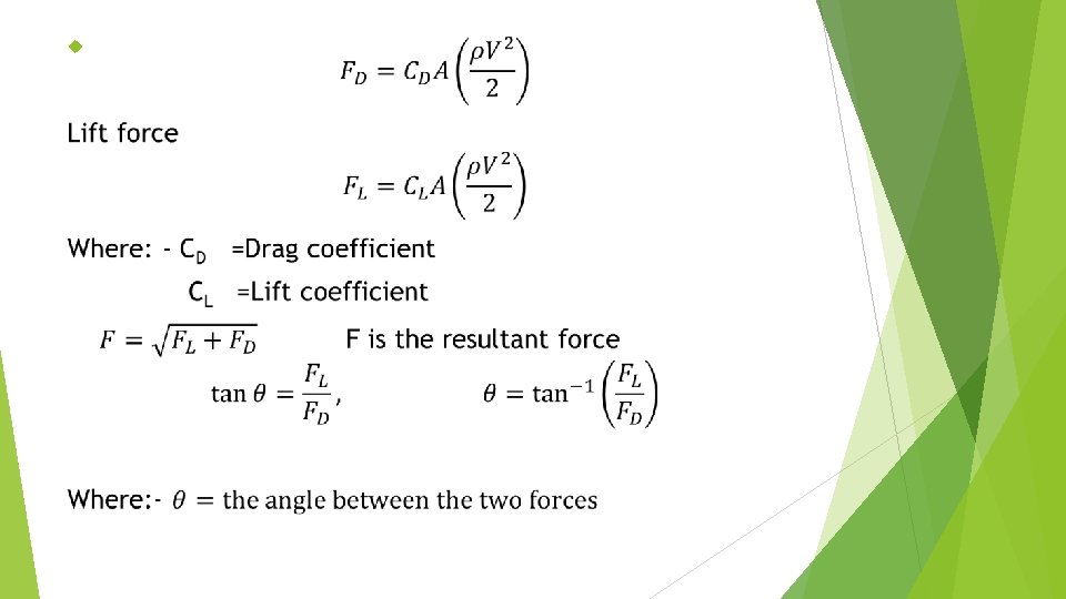
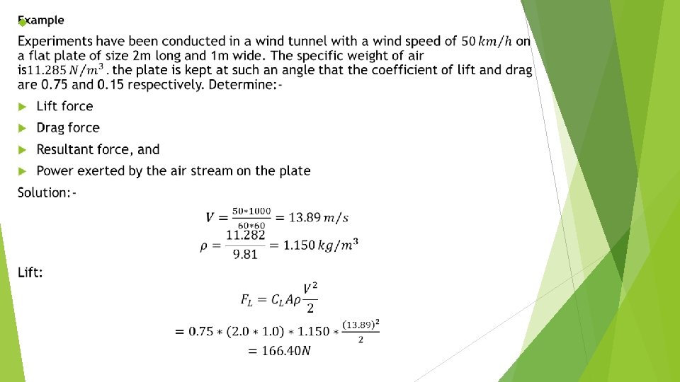
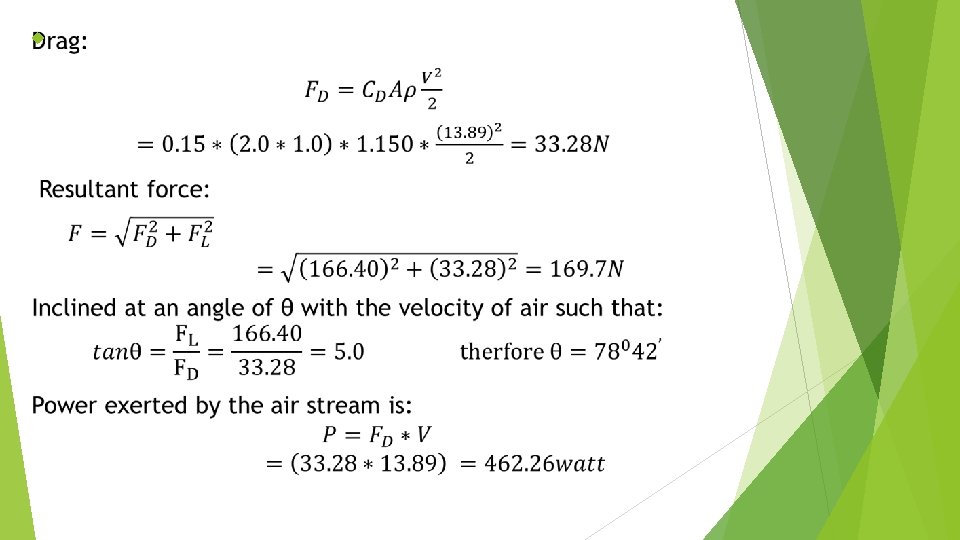
Drag and lift on a sphere and cylinder Take an airfoil immersed in a fluid moving with velocity V

On a sphere

On cylinder- Reading assignment

CHATPER FOUR Laminar and Turbulent Flow Laminar flow: - flow in which the fluid moves in layers, or laminas. Characteristics Re less than 2000. It occurs at Low velocity. The viscous forces predominate over the inertial forces. Rare in practice in water system. Simple mathematical analysis possible.

Turbulent flow: - has very erratic motion of fluid particles, with a violent transverse interchange of momentum. It had completely disrupted the orderly movement of laminar flow. Re greater than 4000. The losses are directly proportional to the average velocity. mathematical analysis is very difficult.

Laminar flow between parallel plates For steady flow b/n parallel inclined plates; the bottom plate fixed, the upper plate has a constant velocity.

Analyzing the flow by taking a thin laminar of unit width as a free body, the equation of motion yields:
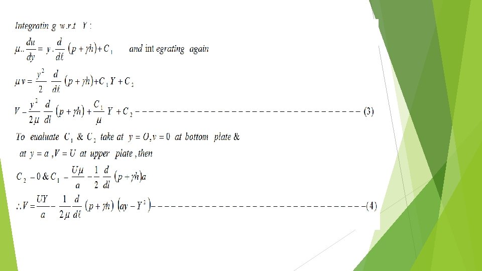

For both plates fixed U=0 The discharge of the laminar flow per unit width of the plate can be obtained by integrating eqn. (4) w. r. t. y, Yielding: For the both plate stationary, U= 0, then,
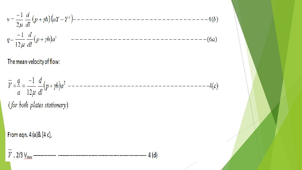
: From the equation")
The shear stress Distribution is given by: Head loss (Energy losses): From the equation (6)

If the flow is laminar in a circular pipe:

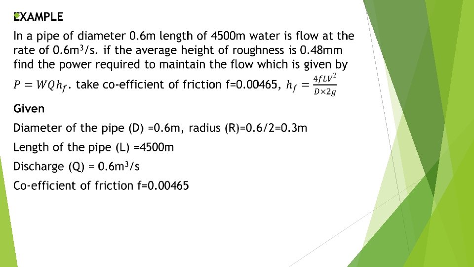
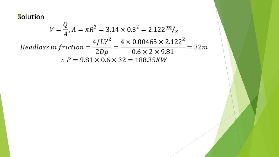
From Darcy- weisbach eqn. the head loss due to frictional resistance in a long straight pipe of length L diameter, D & mean velocity is given as: Note: - The above equations are derived for horizontal pipes, but for inclined pipe it is given as:

Fully developed turbulent flow in pipes Shearing in turbulent flows is both difficult to Visualize & less amenable to mathematical treatment. As consequence, the solutions of problems involving turbulent flows tend to invoke experimental data. In turbulent flow, a streamline broken into an eddy formation, that its success passage leads to a measurable fluctuation in the velocity at a given point. The eddies are generally irregular in size & shape, so the fluctuation of velocity with time is correspondingly irregular.

THANK YOU
- Slides: 41