Chapter ThirtySix Asymmetric Information Information in Competitive Markets

Chapter Thirty-Six Asymmetric Information

Information in Competitive Markets u In purely competitive markets all agents are fully informed about traded commodities and other aspects of the market. u What about markets for medical services, or insurance, or used cars?

Asymmetric Information in Markets u. A doctor knows more about medical services than does the buyer. u An insurance buyer knows more about his riskiness than does the seller. u A used car’s owner knows more about it than does a potential buyer.

Asymmetric Information in Markets u Markets with one side or the other imperfectly informed are markets with imperfect information. u Imperfectly informed markets with one side better informed than the other are markets with asymmetric information.

Asymmetric Information in Markets u In what ways can asymmetric information affect the functioning of a market? u Four applications will be considered: 0 adverse selection 0 signaling 0 moral hazard 0 incentives contracting.

Adverse Selection u Consider a used car market. u Two types of cars; “lemons” and “peaches”. u Each lemon seller will accept $1, 000; a buyer will pay at most $1, 200. u Each peach seller will accept $2, 000; a buyer will pay at most $2, 400.

Adverse Selection u If every buyer can tell a peach from a lemon, then lemons sell for between $1, 000 and $1, 200, and peaches sell for between $2, 000 and $2, 400. u Gains-to-trade are generated when buyers are well informed.

Adverse Selection u Suppose no buyer can tell a peach from a lemon before buying. u What is the most a buyer will pay for any car?

Adverse Selection u Let q be the fraction of peaches. u 1 - q is the fraction of lemons. u Expected value to a buyer of any car is at most

Adverse Selection u Suppose EV > $2000. u Every seller can negotiate a price between $2000 and $EV (no matter if the car is a lemon or a peach). u All sellers gain from being in the market.

Adverse Selection u Suppose EV < $2000. u A peach seller cannot negotiate a price above $2000 and will exit the market. u So all buyers know that remaining sellers own lemons only. u Buyers will pay at most $1200 and only lemons are sold.

Adverse Selection u Hence “too many” lemons “crowd out” the peaches from the market. u Gains-to-trade are reduced since no peaches are traded. u The presence of the lemons inflicts an external cost on buyers and peach owners.

Adverse Selection u How many lemons can be in the market without crowding out the peaches? u Buyers will pay $2000 for a car only if

Adverse Selection u How many lemons can be in the market without crowding out the peaches? u Buyers will pay $2000 for a car only if u So if over one-third of all cars are lemons, then only lemons are traded.

Adverse Selection u. A market equilibrium in which both types of cars are traded and cannot be distinguished by the buyers is a pooling equilibrium. u A market equilibrium in which only one of the two types of cars is traded, or both are traded but can be distinguished by the buyers, is a separating equilibrium.

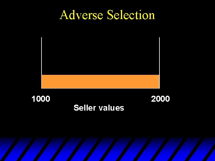
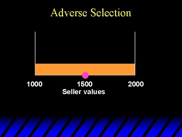
Adverse Selection u What if there is more than two types of cars? u Suppose that 0 car quality is Uniformly distributed between $1000 and $2000 0 any car that a seller values at $x is valued by a buyer at $(x+300). u Which cars will be traded?

Adverse Selection 1000 Seller values 2000

Adverse Selection 1000 1500 Seller values 2000

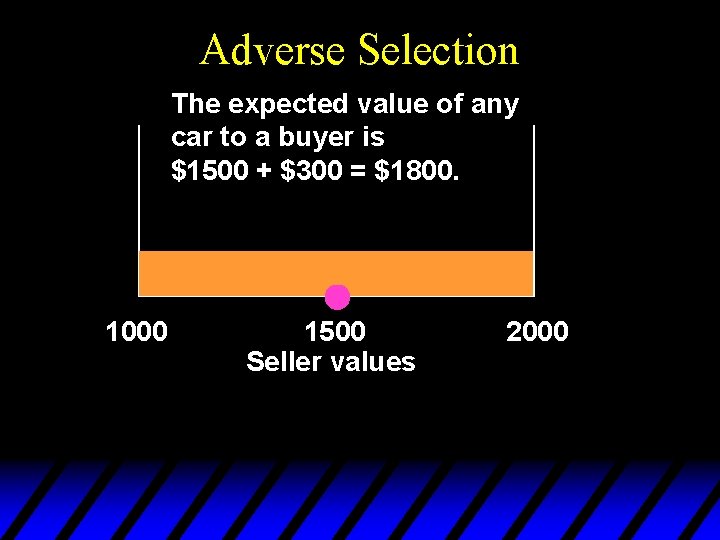
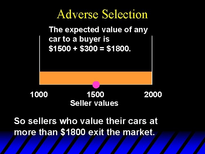
Adverse Selection The expected value of any car to a buyer is $1500 + $300 = $1800. 1000 1500 Seller values 2000

Adverse Selection The expected value of any car to a buyer is $1500 + $300 = $1800. 1000 1500 Seller values 2000 So sellers who value their cars at more than $1800 exit the market.

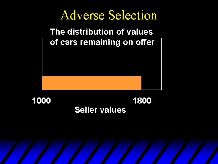
Adverse Selection The distribution of values of cars remaining on offer 1000 Seller values 1800

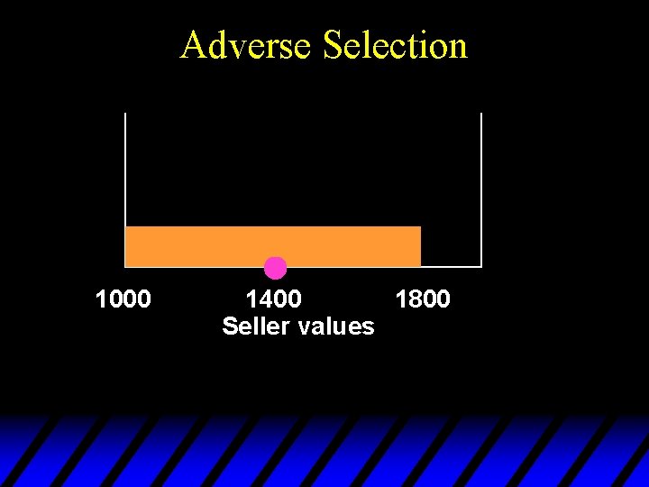
Adverse Selection 1000 1400 1800 Seller values

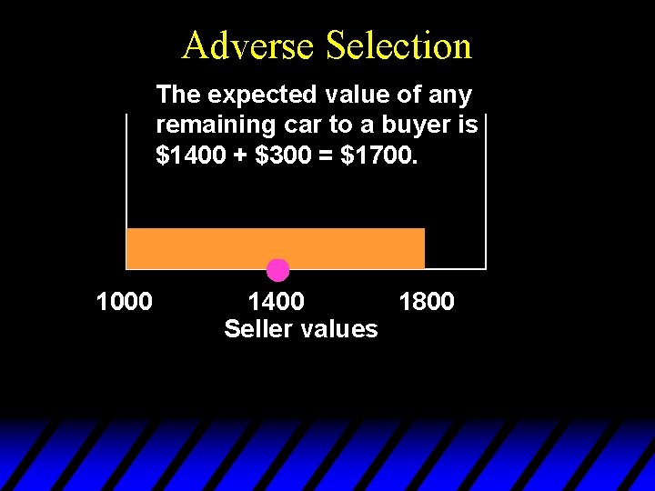
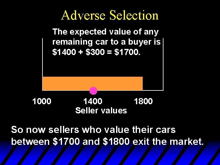
Adverse Selection The expected value of any remaining car to a buyer is $1400 + $300 = $1700. 1000 1400 1800 Seller values

Adverse Selection The expected value of any remaining car to a buyer is $1400 + $300 = $1700. 1000 1400 1800 Seller values So now sellers who value their cars between $1700 and $1800 exit the market.

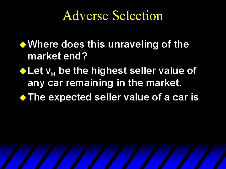
Adverse Selection u Where does this unraveling of the market end? u Let v. H be the highest seller value of any car remaining in the market. u The expected seller value of a car is

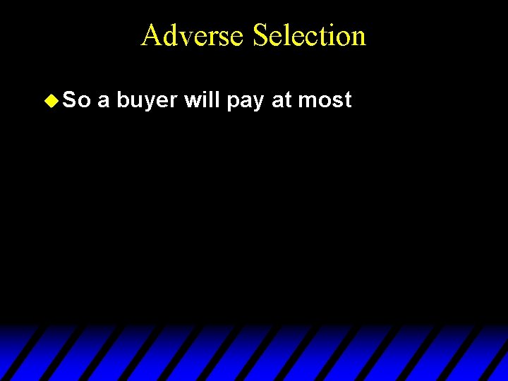
Adverse Selection u So a buyer will pay at most

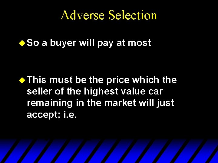
Adverse Selection u So a buyer will pay at most u This must be the price which the seller of the highest value car remaining in the market will just accept; i. e.

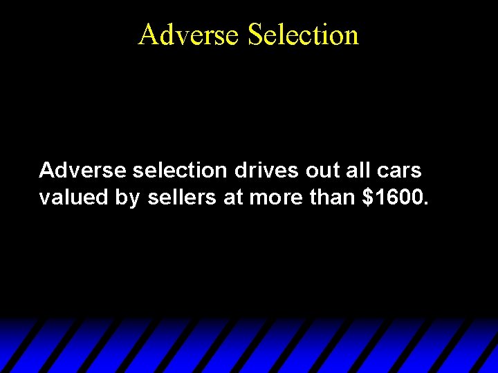
Adverse Selection Adverse selection drives out all cars valued by sellers at more than $1600.

Adverse Selection with Quality Choice u Now each seller can choose the quality, or value, of her product. u Two umbrellas; high-quality and lowquality. u Which will be manufactured and sold?

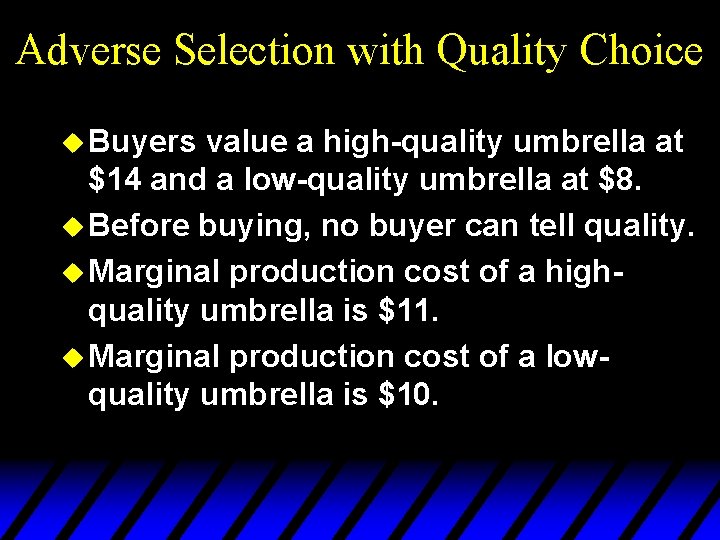
Adverse Selection with Quality Choice u Buyers value a high-quality umbrella at $14 and a low-quality umbrella at $8. u Before buying, no buyer can tell quality. u Marginal production cost of a highquality umbrella is $11. u Marginal production cost of a lowquality umbrella is $10.

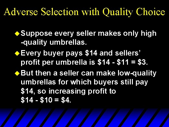
Adverse Selection with Quality Choice u Suppose every seller makes only high -quality umbrellas. u Every buyer pays $14 and sellers’ profit per umbrella is $14 - $11 = $3. u But then a seller can make low-quality umbrellas for which buyers still pay $14, so increasing profit to $14 - $10 = $4.

Adverse Selection with Quality Choice u There is no market equilibrium in which only high-quality umbrellas are traded. u Is there a market equilibrium in which only low-quality umbrellas are traded?

Adverse Selection with Quality Choice u All sellers make only low-quality umbrellas. u Buyers pay at most $8 for an umbrella, while marginal production cost is $10. u There is no market equilibrium in which only low-quality umbrellas are traded.

Adverse Selection with Quality Choice u Now we know there is no market equilibrium in which only one type of umbrella is manufactured. u Is there an equilibrium in which both types of umbrella are manufactured?

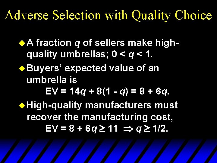
Adverse Selection with Quality Choice u. A fraction q of sellers make highquality umbrellas; 0 < q < 1. u Buyers’ expected value of an umbrella is EV = 14 q + 8(1 - q) = 8 + 6 q. u High-quality manufacturers must recover the manufacturing cost, EV = 8 + 6 q ³ 11 Þ q ³ 1/2.

Adverse Selection with Quality Choice u So at least half of the sellers must make high-quality umbrellas for there to be a pooling market equilibrium. u But then a high-quality seller can switch to making low-quality and increase profit by $1 on each umbrella sold.

Adverse Selection with Quality Choice u Since all sellers reason this way, the fraction of high-quality sellers will shrink towards zero -- but then buyers will pay only $8. u So there is no equilibrium in which both umbrella types are traded.

Adverse Selection with Quality Choice u The market has no equilibrium 0 with just one umbrella type traded 0 with both umbrella types traded

Adverse Selection with Quality Choice u The market has no equilibrium 0 with just one umbrella type traded 0 with both umbrella types traded u so the market has no equilibrium at all.

Adverse Selection with Quality Choice u The market has no equilibrium 0 with just one umbrella type traded 0 with both umbrella types traded u so the market has no equilibrium at all. u Adverse selection has destroyed the entire market!

Signaling u Adverse selection is an outcome of an informational deficiency. u What if information can be improved by high-quality sellers signaling credibly that they are high-quality? u E. g. warranties, professional credentials, references from previous clients etc.

Signaling u. A labor market has two types of workers; high-ability and low-ability. u A high-ability worker’s marginal product is a. H. u A low-ability worker’s marginal product is a. L. u a L < a H.

Signaling u. A fraction h of all workers are highability. u 1 - h is the fraction of low-ability workers.

Signaling u Each worker is paid his expected marginal product. u If firms knew each worker’s type they would 0 pay each high-ability worker w. H = a. H 0 pay each low-ability worker w. L = a. L.

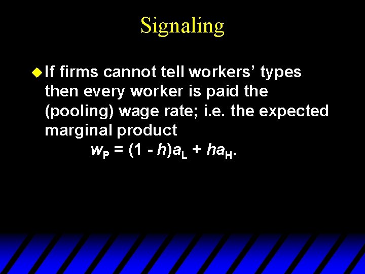
Signaling u If firms cannot tell workers’ types then every worker is paid the (pooling) wage rate; i. e. the expected marginal product w. P = (1 - h)a. L + ha. H.

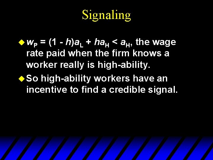
Signaling u w. P = (1 - h)a. L + ha. H < a. H, the wage rate paid when the firm knows a worker really is high-ability. u So high-ability workers have an incentive to find a credible signal.

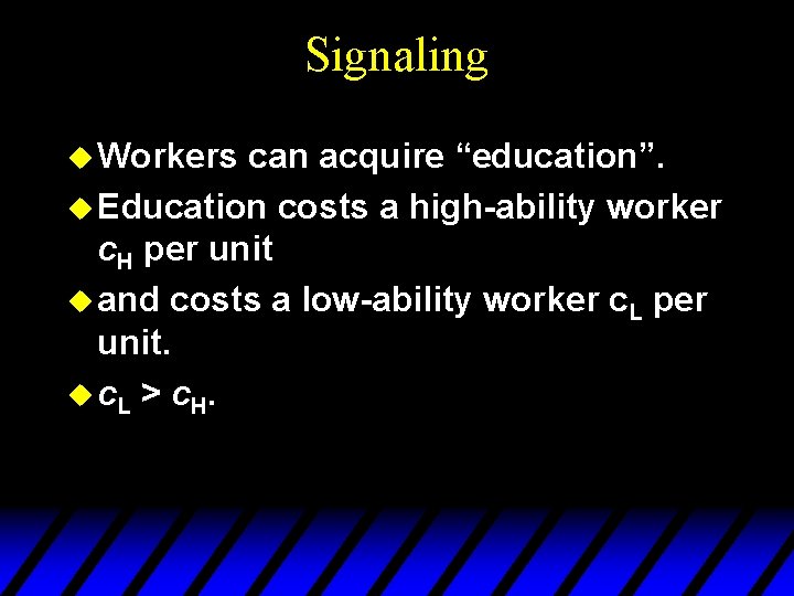
Signaling u Workers can acquire “education”. u Education costs a high-ability worker c. H per unit u and costs a low-ability worker c. L per unit. u c L > c H.

Signaling u Suppose that education has no effect on workers’ productivities; i. e. , the cost of education is a deadweight loss.

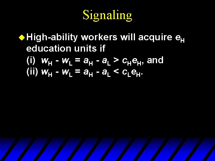
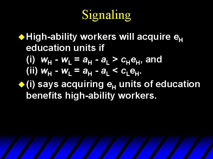
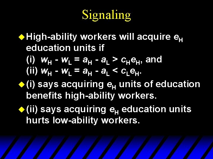
Signaling u High-ability workers will acquire e. H education units if (i) w. H - w. L = a. H - a. L > c. He. H, and (ii) w. H - w. L = a. H - a. L < c. Le. H.

Signaling u High-ability workers will acquire e. H education units if (i) w. H - w. L = a. H - a. L > c. He. H, and (ii) w. H - w. L = a. H - a. L < c. Le. H. u (i) says acquiring e. H units of education benefits high-ability workers.

Signaling u High-ability workers will acquire e. H education units if (i) w. H - w. L = a. H - a. L > c. He. H, and (ii) w. H - w. L = a. H - a. L < c. Le. H. u (i) says acquiring e. H units of education benefits high-ability workers. u (ii) says acquiring e. H education units hurts low-ability workers.

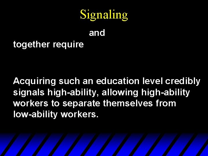
Signaling and together require Acquiring such an education level credibly signals high-ability, allowing high-ability workers to separate themselves from low-ability workers.

Signaling u Q: Given that high-ability workers acquire e. H units of education, how much education should low-ability workers acquire?

Signaling u Q: Given that high-ability workers acquire e. H units of education, how much education should low-ability workers acquire? u A: Zero. Low-ability workers will be paid w. L = a. L so long as they do not have e. H units of education and they are still worse off if they do.

Signaling u Signaling can improve information in the market. u But, total output did not change and education was costly so signaling worsened the market’s efficiency. u So improved information need not improve gains-to-trade.

Moral Hazard u If you have full car insurance are you more likely to leave your car unlocked? u Moral hazard is a reaction to incentives to increase the risk of a loss u and is a consequence of asymmetric information.

Moral Hazard u If an insurer knows the exact risk from insuring an individual, then a contract specific to that person can be written. u If all people look alike to the insurer, then one contract will be offered to all insurees; high-risk and low-risk types are then pooled, causing lowrisks to subsidize high-risks.

Moral Hazard u Examples of efforts to avoid moral hazard by using signals are: 0 higher life and medical insurance premiums for smokers or heavy drinkers of alcohol 0 lower car insurance premiums for contracts with higher deductibles or for drivers with histories of safe driving.

Incentives Contracting u. A worker is hired by a principal to do a task. u Only the worker knows the effort she exerts (asymmetric information). u The effort exerted affects the principal’s payoff.

Incentives Contracting u The principal’s problem: design an incentives contract that induces the worker to exert the amount of effort that maximizes the principal’s payoff.

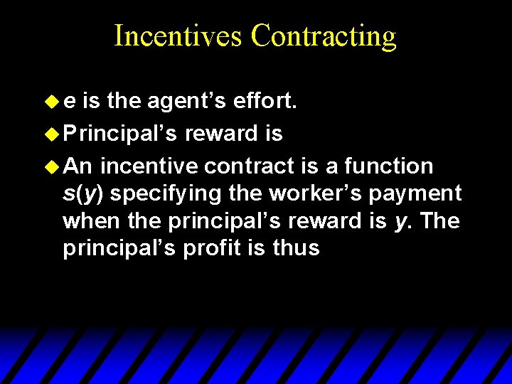
Incentives Contracting ue is the agent’s effort. u Principal’s reward is u An incentive contract is a function s(y) specifying the worker’s payment when the principal’s reward is y. The principal’s profit is thus

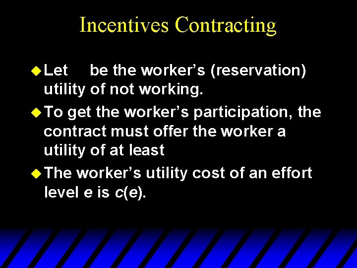
Incentives Contracting u Let be the worker’s (reservation) utility of not working. u To get the worker’s participation, the contract must offer the worker a utility of at least u The worker’s utility cost of an effort level e is c(e).

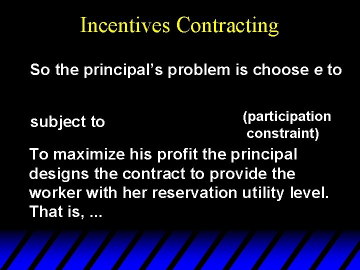
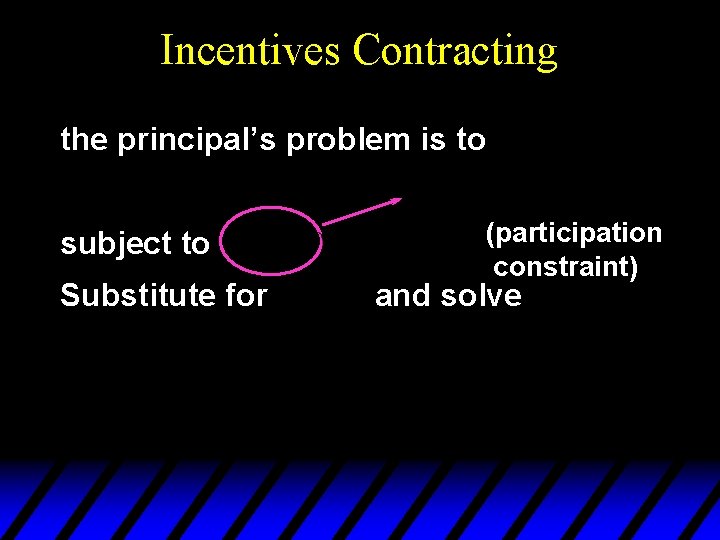
Incentives Contracting So the principal’s problem is choose e to subject to (participation constraint) To maximize his profit the principal designs the contract to provide the worker with her reservation utility level. That is, . . .

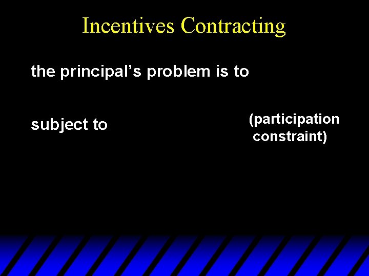
Incentives Contracting the principal’s problem is to subject to (participation constraint)

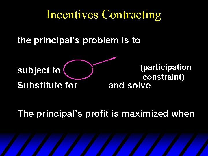
Incentives Contracting the principal’s problem is to subject to Substitute for (participation constraint) and solve

Incentives Contracting the principal’s problem is to subject to Substitute for (participation constraint) and solve The principal’s profit is maximized when

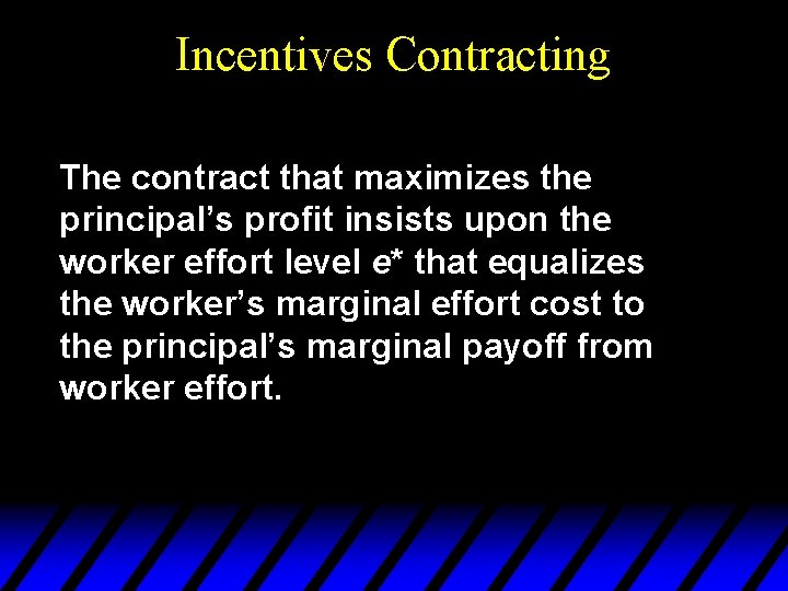
Incentives Contracting The contract that maximizes the principal’s profit insists upon the worker effort level e* that equalizes the worker’s marginal effort cost to the principal’s marginal payoff from worker effort.

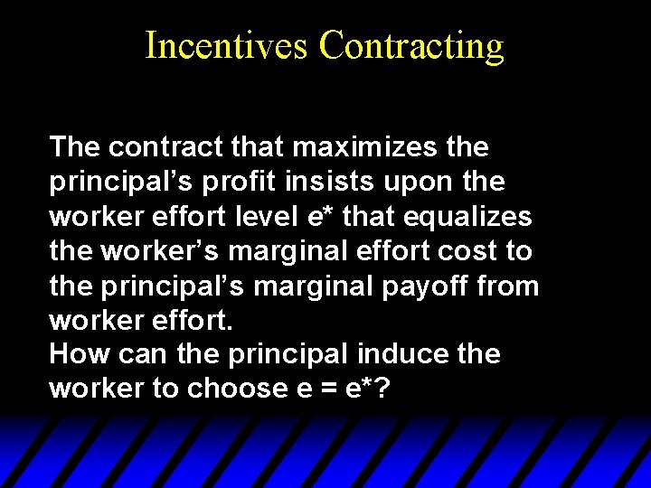
Incentives Contracting The contract that maximizes the principal’s profit insists upon the worker effort level e* that equalizes the worker’s marginal effort cost to the principal’s marginal payoff from worker effort. How can the principal induce the worker to choose e = e*?

Incentives Contracting ue = e* must be most preferred by the worker.

Incentives Contracting ue = e* must be most preferred by the worker. u So the contract s(y) must satisfy the incentive-compatibility constraint;

Rental Contracting u Examples of incentives contracts: (i) Rental contracts: The principal keeps a lump-sum R for himself and the worker gets all profit above R; i. e. u Why does this contract maximize the principal’s profit?

Rental Contracting u Given the contract the worker’s payoff is and to maximize this the worker should choose the effort level for which

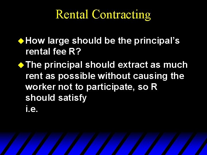
Rental Contracting u How large should be the principal’s rental fee R? u The principal should extract as much rent as possible without causing the worker not to participate, so R should satisfy i. e.

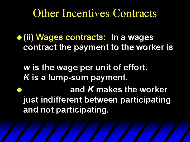
Other Incentives Contracts u (ii) Wages contracts: In a wages contract the payment to the worker is w is the wage per unit of effort. K is a lump-sum payment. u and K makes the worker just indifferent between participating and not participating.

Other Incentives Contracts u (iii) Take-it-or-leave-it: Choose e = e* and be paid a lump-sum L, or choose e ¹ e* and be paid zero. u The worker’s utility from choosing e ¹ e* is - c(e), so the worker will choose e = e*. u L is chosen to make the worker indifferent between participating and not participating.

Incentives Contracts in General u The common feature of all efficient incentive contracts is that they make the worker the full residual claimant on profits. u I. e. the last part of profit earned must accrue entirely to the worker.