Chapter Six Wind Energy Systems Modern Applications of

Chapter Six Wind Energy Systems

• Modern Applications of Wind Energy • Considering its end use applications, wind energy generation are classified as: ü Off-grid applications; and ü On-grid applications. Off- grid applications Ø Wind energy is competitive in remote sites, far from the electric grid, requiring relatively small amounts of power. Ø Wind energy can be used to charge batteries. Ø Wind energy can be used in water pumping. Ø Small turbines (50 W to 10 k. W) On-Grid Applications • Wind energy system feeds electrical energy directly into the electric utility grid.

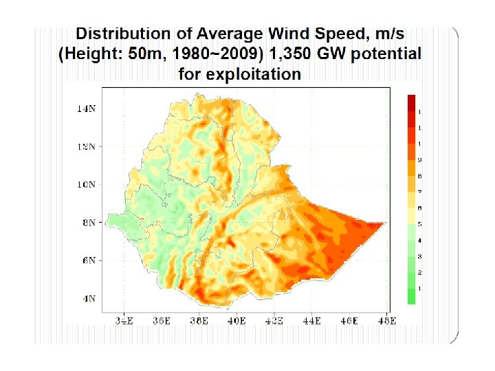
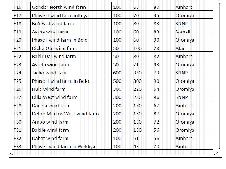
• Wind Energy in Ethiopia • The government of Ethiopia with collaboration of Chinese government prepared solar and wind master plan for the whole country. • Based on the analysis of this master plan: • Ethiopia has a capacity of 1, 350 GW of energy from wind. • Generally, the overall wind potential of the country is approximated to be about 10 GW However, even though the available potentials were spotted decades ago, it is not until very recently that its practical development caught the attention of the concerned body.

Characteristics of Wind Ø Wind is stochastic in nature. Speed and direction of wind at a location vary randomly with time. Apart from the daily and seasonal variations, the wind pattern may change from year to year, even to the extent of 10 to 30 per cent. Ø Hence, the behavior of the wind at a prospective site should be properly analyzed and understood. Ø Realizing the nature of wind is important for a designer, as he can design his turbine and its components in tune with the wind characteristics expected at the site. Ø Similarly, a developer can assess the energy that could be generated from his project, if the wind regime characteristics are known.

Ø wind is generated due to the pressure gradient resulting from the uneven heating of earth’s surface by the sun. Ø As the very driving force causing this movement is derived from the sun, wind energy is basically an indirect form of solar energy. Ø One to two per cent of the total solar radiation reaching the earth’s surface is converted to wind energy in this way. Ø The wind described above, which is driven by the temperature difference, is called the geostrophic wind, or more commonly the global wind. Ø Global winds, which are not affected by the earth surface, are found at higher altitudes.

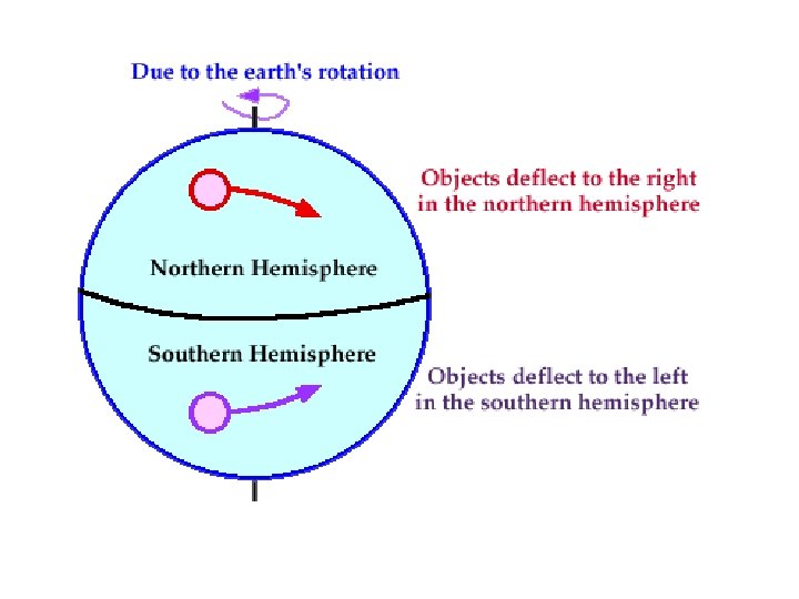
Ø Due to the Coriolis effect (due to rotation of earth) , the straight movement of air mass from the high pressure region to the low pressure region is diverted as shown in Fig. below. Under the influence of Coriolis forces, the air move almost parallel to the isobars. Thus, in the northern hemisphere, wind tends to rotate clockwise where as in the southern hemisphere the motion is in the anti -clockwise direction. Fig. Wind direction affected by the Coriolis force

Mean Annual Wind Speed and Wind Speed Frequency Distribution Ø Apart from the average strength of wind over a period, its distribution is also a critical factor in wind resource assessment. Ø Wind turbines installed at two sites with the same average wind speed may yield entirely different energy output due to differences in the velocity distribution. Ø One measure for the variability of velocities in a given set of wind data is the standard deviation ( v). Standard deviation tells us the deviation of individual velocities from the mean value. Thus

Ø For a better understanding on wind variability, the data are often grouped and presented in the form of frequency distribution. Ø This gives us the information on the number of hours for which the velocity is within a specific range. Ø For developing the frequency distribution, the wind speed domain is divided into equal intervals (say 0 -1, 1 -2, 2 -3, etc. ) and the number of times the wind record is within this interval is counted. Ø If the velocity is presented in the form of frequency distribution, the average and standard deviation are given by

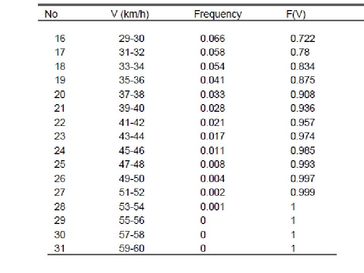
Example: Frequency distribution of monthly wind velocity

Probability distribution of monthly wind velocity

The average and standard deviation of wind data presented in previous table are 8. 34 m/s and 0. 81 m/s respectively. Frequency histogram based on the above data is shown in previous Fig. It is interesting to note that, the average wind speed does not coincide with the most frequent wind speed. Cumulative distribution of wind velocity

Increase in wind speed with Altitude – Wind Shear Ø The flow of air above the ground is retarded by frictional resistance offered by the earth surface (boundary layer effect). This resistance may be caused by the roughness of the ground itself or due to vegetations, buildings and other structures present over the ground. Wind speed generally increases with height (z) in the atmospheric boundary layer

Ø Typical vertical wind profile at a site is shown in Fig. below. Theoretically, the velocity of wind right over the ground surface should be zero. Velocity increases with height up to a certain elevation. Fig. Variation of wind velocity with height

Ø The rate at which the velocity increases with height depends on the roughness of the terrain. Presence of dense vegetations like plantations, forests, and bushes slows down the wind considerably. Ø The surface roughness of a terrain is usually represented by the roughness class or roughness height. The roughness height of a surface may be close to zero (surface of the sea) or even as high as 2 (town centers). Terrain type Roughness height Flat and smooth terrains 0. 005 Open grass lands 0. 025 -0. 1 Row crops 0. 2 -0. 3 Orchards and shrubs 0. 5 -1. 0 Forests, town centers 1. 0 -2. 0

Ø Roughness height is an important factor to be considered in the design of wind energy plants. • In wind energy calculations, we are concerned with the velocity available at the rotor height. • The data collected at any heights can be extrapolated to other heights on the basis of the roughness height of the terrain. Ø Due to the boundary layer effect, wind speed increases with the height in a logarithmic pattern. If the wind data is available at a height Z and the roughness height is Z 0, then the velocity at a height ZR is given by: 6. 1 where V (ZR) and V(Z) are the velocities at heights ZR and Z respectively

Ø In some cases, we may have data from a reference location (meteorological station for example) at a certain height. This data is to be transformed to a different height at another location with similar wind profile but different roughness height (for example, the wind turbine site). Ø Under such situations, it is logical to assume that the wind velocity is not significantly affected by the surface characteristics beyond a certain height. This height may be taken as 60 m from the ground level. Thus, expressing the velocity at 60 m in terms of the reference location, 6. 2

Turbulence Ø Turbulence refers to fluctuations in wind speed on a relatively fast time-scale, typically less than about 10 min. speed and direction of wind change rapidly while it passes through surfaces and obstructions like buildings, trees and rocks. This is due to the turbulence generated in the flow. Ø Extent of this turbulence at the upstream and downstream of the flow is shown in Fig. below. The presence of turbulence in the flow not only reduces the power available in the stream, but also imposes fatigue loads on the turbine. Fig. Turbulence created by an obstruction

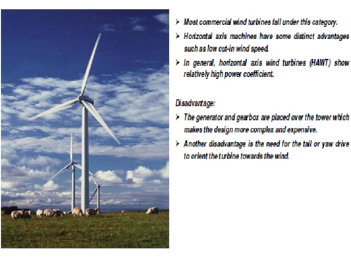
Classification of wind turbines Ø Since the inception of the wind energy technology, machines of several types and shapes were designed and developed around different parts of the world. Ø Although there are several ways to categorize wind turbines, they are broadly classified into horizontal axis machines and vertical axis machines, based on their axis of rotation. Horizontal axis wind turbines Ø Horizontal axis wind turbines (HAWT) have their axis of rotation horizontal to the ground almost parallel to the wind stream.

Fig. Horizontal axis wind turbines

• Depending on the number of blades, horizontal axis wind turbines are further classified as single bladed, two bladed, three bladed and multi bladed, as shown in Fig. below. Fig. Classification of wind turbines by number of blades Single bladed turbines are cheaper due to savings on blade materials. The drag losses are also minimum for these turbines. How ever to balance the blade, a counter weight has to be placed opposite to the hub. Single bladed designs are not very popular due to problems in balancing and visual acceptability.

• Two bladed rotors also have these drawbacks, but to a lesser extent. Most of the present commercial turbines used for electricity generation have three blades. • Machines with more number of blades (6, 8, 12, 18 or even more) are also available. • The ratio between the actual blade area to the swept area of a rotor is termed as the solidity. Hence, multi-bladed rotors are also called high solidity rotors. • High solidity rotors can start easily as more rotor area interacts with the wind initially. Some low solidity designs may require external starting.

• Question: Then why do we need turbines with more blades? • Answer: Some applications like water pumping require high starting torque. For such systems, the torque required for starting goes up to 3 -4 times the running torque. Starting torque increases with the solidity. Hence to develop high starting torque, water pumping wind mills are made with multi bladed rotors.

Vertical axis wind turbines • The axis of rotation of vertical axis wind turbine (VAWT) is vertical to the ground almost perpendicular to the wind direction as seen from Fig. below Fig. Vertical Axis wind turbine The VAWT can receive wind from any direction. Hence complicated yaw devices can be eliminated. - generator and the gearbox housed at the ground level, which makes the tower design simple and more economical. Moreover - the maintenance of these turbines can be done at the ground level.

• The major disadvantage of some VAWT are - they are usually not self starting. Additional mechanisms may be required to ‘push’ and start the turbine, once it is stopped. -There are chances that the blades may run at dangerously high speeds causing the system to fail, if not controlled properly. -guy wires are required to support the tower structure which may pose practical difficulties. Reading Assignment about types of VAWT • Darrieus rotor • Savonius rotor • Musgrove rotor

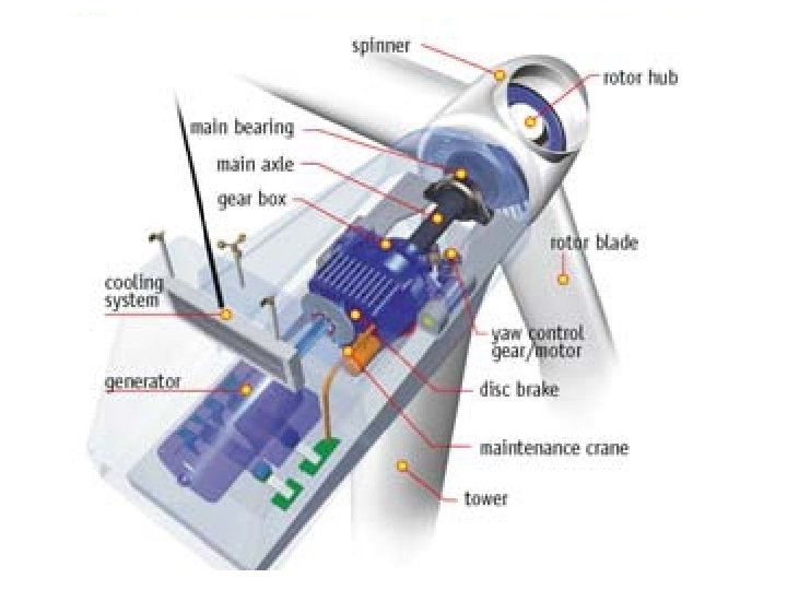
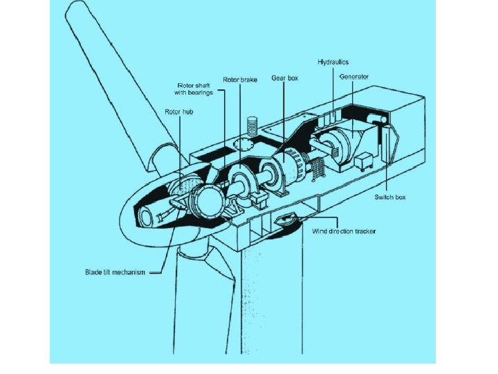
• Wind Turbine Subsystems Foundation – Tower – Nacelle – Hub & Rotor – Drivetrain – Gearbox – Generator – Electronics & Controls – Yaw – Pitch – Braking – Power Electronics – Cooling – Diagnostics

Fig Components of a Wind Electric Generator

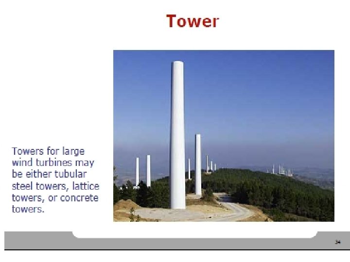
Tower • Tower supports the rotor and nacelle of a wind turbine at the desired height. • major types of towers used in modern turbines are lattice tower, tubular steel tower and guyed tower. Schematic views of these towers are shown in Fig. below. Fig. Different types of towers

• The lattice towers are fabricated with steel bars joined together to form the structure as shown in the figure. They are similar to the transmission towers of electric utilities. • Lattice towers consume only half of the material that is required for a similar tubular tower. As the load is distributed over a wider area, these towers require comparatively lighter foundation, which will again contribute to the cost reduction. • Lattice towers are not maintenance friendly. At installations where the temperature drops to an extremely low level, maintenance of systems with lattice towers is difficult as workers would be exposed to the chilling weather. • Moreover, as these towers do not have any lockable doors, they are less secure for maintenance.

• Due to these limitations, most of the recent installations are provided with tubular steel towers. • These towers are fabricated by joining tubular sections of 10 to 20 m length. The complete tower can be assembled at the site. • The tubular tower, with its circular cross-section, can offer optimum bending resistance in all directions. • These towers are aesthetically acceptable and pose less danger to the avian population. • For small systems, towers with guyed steel poles are being used. By partially supporting the turbine on guy wires, weight and thus the cost of the tower can be considerably reduced. Usually, four cables equally spaced and inclined at 45 o, support the tower.

• Wind velocity increases with height due to wind shear. Hence, the taller the tower, the higher will be the power available to the rotor. Rate at which the available power increases with height depends on the surface roughness of the ground. • The performance of a wind turbine improves with its tower height. However, taller towers cost more. • Towers account for around 20 per cent of the total systems cost. At present, cost of every additional 10 m of tower is approximately $15, 000. • Can the additional cost be justified by the improvement in system performance? In other words, what should be the optimum tower height? • The best criterion is to work out the economics of the options in terms of cost per k. Wh of electricity generated.

Rotor • Rotor is the most important and prominent part of a wind turbine. Components of a wind turbine rotor are blades, hub, shaft, bearings and other internals. • Size of the rotor depends on the power rating of the turbine. The turbine cost, in terms of $ per rated k. W, decreases with the increase in turbine size. Hence, MW sized designs are getting popular in the industry. • Blades are fabricated with a variety of materials ranging from wood to carbon composites. Use of wood and metal are limited to small scale units. Most of the large scale commercial systems are made with multi layered fiberglass blades.

Four sides of a rotor blade of a wind turbine

• The blades of the rotor are attached to hub assembly. The hub assembly consists of hub, bolts, blade bearings, pitch system and internals. • Hub is one of the critical components of the rotor requiring high strength qualities. They are subjected to repetitive loading due to the bending moments of the blade root. • Due to the typical shape of the hub and high loads expected, it is usually cast in special iron alloys like the spherical graphite (SG) cast iron. • Forces acting on the hub make its design a complex process. Three dimensional Finite Element Analysis (FEA) and topological optimization techniques are being effectively used for the optimum design of the hub assembly.

• The main shaft of the turbine passes through the main bearings. Roller bearings are commonly used for wind turbines. • These bearings can tolerate slight errors in the alignment of the main shaft, thus eliminating the possibility of excessive edge loads. • The bearings are lubricated with special quality grease which can withstand adverse climatic conditions. • Replacing the bearings of an installed turbine is a very costly work. Hence, to ensure longer life and reliable performance, hybrid ceramic bearings are used with some recent designs. • The advantages of ceramic hybrids are that they are stiffer, harder and corrosion free and can sustain adverse operating conditions.

Gearbox • The power from the rotation of the wind turbine rotor is transferred to the generator through the power train, i. e. through the main (low speed) shaft, the gearbox and the high speed shaft. • Gear box is an important component in the power trains of a wind turbine. Speed of a typical wind turbine rotor may be 30 to 50 r/min whereas, the optimum speed of generator may be around 1000 to 1500 r/min. • Hence, gear trains are to be introduced in the transmission line to manipulate the speed according to the requirement of the generator.

• In smaller turbines, the desired speed ratio is achieved by introducing two or three staged gearing system. • For example, the gear arrangement in a 150 k. W turbine is shown in the Fig. below. Fig. Gear arrangements of a small wind turbine

• Here, the rotational speed of the rotor is around 40 r/min whereas the generator is designed to operate at 1000 r/min. Thus a gear ratio of 25 is required, which is accomplished in two stages as shown in the figure. • Low speed shaft from the rotor carries a bigger gear which drives a smaller gear on the intermediate shaft. Teeth ratio between the bigger and smaller gear is 1: 5 and thus the intermediate shaft rotates 5 times faster than the low speed shaft. • The speed is further enhanced by introducing the next set of gear combination with bigger gear on the intermediate shaft driving a smaller gear on the generator shaft. Finally the desired 1: 25 gear ratio is achieved.

• If higher gear ratios are required, a further set of gears on another intermediate shaft can be introduced in the system. However, the ratio between a set of gears are normally restricted to 1: 6. • An ideal gear system should be designed to work smoothly and quietly-even under adverse climatic and loading conditions-throughout the life span of the turbine. • Due to special constraints in the nacelle, the size is also a critical factor.

Power available in the wind spectra Ø Consider a wind rotor of cross sectional area A exposed to a wind stream as shown in Fig. below. The kinetic energy of the air stream available for the turbine can be expressed 6. 3 as: Fig. An air parcel moving towards a wind turbine

The air parcel interacting with the rotor per unit time has a cross-sectional area equal to that of the rotor (AT) and thickness equal to the wind velocity (V). Hence energy per unit time, that is power, can be expressed as: 6. 4 From Eq. (6. 4), we can see that the factors influencing the power available in the wind stream are the air density, area of the wind rotor and the wind velocity. If we know the elevation Z and temperature T at a site, then the air density can be calculated by: 6. 5

Fig. Effect of elevation and temperature on air density Due to the relatively low density (~1. 225 kg/m 3), wind is rather a diffused source of energy. Hence large sized systems are often required for substantial power production.

Ø The most prominent factor deciding the power available in the wind spectra is its velocity. When the wind velocity is doubled, the available power increases by 8 times. In other words, for the same power, rotor area can be reduced by a factor of 8, if the system is placed at a site with double the wind velocity. Ø Hence, selecting the right site play a major role in the success of a wind power projects.

Wind turbine power and torque Ø When the wind stream passes the turbine, a part of its kinetic energy is transferred to the rotor and the air leaving the turbine carries the rest away. Ø Actual power produced by a rotor would be decided by the efficiency with which the energy transfer from wind to the rotor takes place. This efficiency is usually termed as the power coefficient (Cp). Ø the power coefficient of the rotor can be defined as the ratio of actual power developed by the rotor to theoretical power available in the wind. 6. 7 where PT is the power developed by the turbine.

• Power extracted from the wind (Albert Betz’s Formulation) Assume that the velocity of wind vb is just the average of the upwind and downwind speed,

Denote the ratio between upwind and downwind speed by: Substitute vd, then we have, 6. 8 Comparing equation 6. 7 and 6. 8 reveals that the last term is the power coefficient or rotor efficiency. 6. 9 Variation of power coefficient with speed ratio is shown in next figure. The question is to identify the speed ratio which gives maximum efficiency

How should we design λ so that we can have better rotor efficiency?

• The blade efficiency will be maximum if it slows the wind to one-third of the upwind speed, 6. 10 We can now find the maximum rotor efficiency (power coefficient) 6. 11

Ø The thrust force experienced by the rotor (F) can be expressed as: 6. 12 and the rotor torque (T) is 6. 13 where R is the radius of the rotor. Thus, the torque coefficient is given by 6. 14 where TT is the actual torque developed by the rotor.

Tip-Speed Ratio Ø The power developed by a rotor at a certain wind speed greatly depends on the relative velocity between the rotor tip and the wind. Ø For a given wind speed, rotor efficiency is a function of the rate at which a rotor turn. -Rotor turns too slow letting too much wind pass -> efficiency drop. –Rotor turns too fast causing turbulence -> efficiency drop. The ratio between the velocity of the rotor tip and the wind velocity is termed as the tip speed ratio ( ). Thus, 6. 15

Ø The power coefficient and torque coefficient of a rotor vary with the tip speed ratio. There is an optimum for a given rotor at which the energy transfer is most efficient and thus the power coefficient is the maximum (CP max).

• Note that the tip speed ratio is also given by the ratio between the power coefficient and torque coefficient of the rotor. 6. 16 Example Consider a wind turbine with 5 m diameter rotor. Speed of the rotor at 10 m/s wind velocity is 130 r/min and its power coefficient at this point is 0. 35. Calculate the tip speed ratio and torque coefficient of the turbine. What will be the torque available at the rotor shaft? Assume the density of air to be 1. 24 kg/m 3.

Exercise • A 40 -m, three-bladed wind turbine produces 600 k. W at a wind speed of 14 m/s. Air density is the standard 1. 225 kg/m 3. Under these conditions, a. At what rpm does the rotor turn when it operates with a TSR of 4. 0? b. What is the tip speed of the rotor? c. If the generator needs to turn at 1800 rpm, what gear ratio is needed to match the rotor speed to the generator speed? d. What is the efficiency of the complete wind turbine (blades, gear box, generator) under these conditions?

Statistical models for wind data analysis • Various probability functions were fitted with the field data to identify suitable statistical distributions for representing wind regimes. • It is found that the Weibull and Rayleigh distributions can be used to describe the wind variations in a regime with an acceptable accuracy level • Weibull distribution • In Weibull distribution, the variations in wind velocity are characterized by the two functions; • (1) The probability density function and • (2) The cumulative distribution function.

probability density function • The probability density function (f(V)) indicates the fraction of time (or probability) for which the wind is at a given velocity V. It is given by 6. 17 Here, k is the Weibull shape factor and c is scale factor. cumulative distribution function The cumulative distribution function of the velocity V gives us the fraction of time (or probability) that the wind velocity is equal or lower than V. Thus the cumulative distribution F(V) is the integral of the probability density function. Thus,

6. 18 Average wind velocity of a regime, following the Weibull distribution is given by 6. 19 Substituting for f(V)) we get 6. 20 which can be rearranged as 6. 21

• Taking Substituting for d. V in Eq. 6. 21 6. 22 Eq. 6. 22 is in the form of the standard gamma function, which is given by 6. 23 Hence, from Eq. (6. 22), the average velocity can be expressed as 6. 24

• The standard deviation of wind velocity, following the Weibull distribution is 6. 25 The probability density and cumulative distribution functions of a wind regime following the Weibull distribution are shown in Fig. 6. 3 and 6. 4 The k and c values for this site are 2. 8 and 6. 9 m/s respectively. The peak of the probability density curve indicates the most frequent wind velocity in the regime, which is 6 m/s in this case.

Fig. 6. 3. Weibull probability density function

Fig. 6. 4. Weibull cumulative distribution function

The cumulative distribution function can be used for estimating the time for which wind is within a certain velocity interval. Probability of wind velocity being between V 1 and V 2 is given by the difference of cumulative probabilities corresponding to V 2 and V 1. Thus 6. 26 That is 6. 27 We may be interested to know the possibilities of extreme wind at a potential location, so that the system can be designed to sustain the maximum probable loads. The probability for wind exceeding VX in its velocity is given by 6. 28

• Example 1 • A wind turbine with cut-in velocity 4 m/s and cutout velocity 25 m/s is installed at a site with Weibull shape factor 2. 4 and scale factor 9. 8 m/s. For how many hours in a day, will the turbine generate power? Also estimate the probability of wind velocity to exceed 35 m/s at this site.

• Under the Weibull distribution, the major factor determining the uniformity of wind is the shape factor k. Figures 6. 5 and 6. 6 illustrate the effect of k on the probability density and cumulative distribution functions of wind. Here, the scale factor is taken as 9. 8 m/s. • Uniformity of wind at the site increases with k. • For example, with k =1. 5, the wind velocity is between 0 and 20 m/s for 95 per cent of the time. Whereas, when k = 4, the velocity is more evenly distributed within a smaller range of 0 to 13 m/s for 95 per cent of the time. In the first case, the most frequent wind speed is 5 m/s, which is expected for 7. 6 per cent of the total time. • The most frequent wind speed of 9 m/s would prevail for 15. 5 per cent of the time in the second case.

Fig. 6. 5. Weibull probability density function for different shape factors

Fig. 6. 6. Weibull probability density function for different shape factors

• For analyzing a wind regime following the Weibull distribution, we have to estimate the Weibull parameters k and c. The common methods for determining k and c are: 1. Graphical method 2. Standard deviation method 3. Moment method 4. Maximum likelihood method and 5. Energy pattern factor method • Here, only Graphical and Standard deviation methods are discussed.

Graphical method • In the graphical method, we transform the cumulative distribution function in to a linear form, adopting logarithmic scales. • The expression for the cumulative distribution of wind velocity can be rewritten as 6. 29 Taking the logarithm twice, we get 6. 30 Plotting the above relationship with ln (Vi) along the X axis and ln{-ln[1 -F(V)]} along the Y axis, we get nearly a straight line. From Eq. (6. 30), k gives the slope of this line and –k ln c represents the intercept.

Example 2 • The frequency distribution of wind velocity at a site is given in Table below. Calculate the Weibull shape and scale factors.

• First of all, we have to generate the cumulative distribution of the data based on the given frequencies. Each class should be represented by its upper limit as shown in the last column of the table. • Now plot ln (V) in the X axis and ln {-ln [1 - F(V)]} in the Y axis. • The resulting equation for the plot is The coefficient of determination (R 2) between the data and the fitted line is 0. 98. Comparing the resulting equation with Eq. (6. 30), we get k for the given location as 2. 24. Similarly, we have k ln c = 7. 32. From this c can be solved as 26. 31 km/h (7. 31 m/s).

Fig. 6. 7 Graphical method to estimate Weibull k and c (for the above example)

Standard deviation method • The Weibull factors k and c can also be estimated from the mean and standard deviation of wind data. Consider the expressions for average and standard deviation derived previously. We have: 6. 31 Once V and Vm are calculated for a given data set, then k can be determined by solving the above expression numerically. Once k is determined, c is given by 6. 32

• In a simpler approach, an acceptable approximation for k is 6. 33 Similarly, c can be approximated as 6. 34 More accurately, c can be found using the expression 6. 35

• Example 3 • Estimate the Weibull factors k and c for the data in Example 2 using the standard deviation method. • Solution: Mean and standard deviation of the given data, as per the following equations are 28. 08 km/h (7. 80 m/s) and 10. 88 km/h (3. 02 m/s) respectively. Thus Substituting for Vm and k in Eq. (6. 35),

• We can see that, there are differences in k and c estimated, following the graphical and standard deviation methods. The cumulative distributions generated using these methods are compared with the field measurements (represented by dotted lines) in Fig. 6. 8 Cumulative distribution generated using different methods

Rayleigh distribution • The reliability of Weibull distribution in wind regime analysis depends on the accuracy in estimating k and c. • For the precise calculation of k and c, adequate wind data, collected over shorter time intervals are essential. • In many cases, such information may not be readily available. The existing data may be in the form of the mean wind velocity over a given time period (for example daily, monthly or yearly mean wind velocity). • Under such situations, a simplified case of the Weibull model can be derived, approximating k as 2. This is known as the Rayleigh distribution.

• Taking k = 2 in Eq. (3. 8) we get 6. 36 Evaluating the above expression and rearranging, 6. 37 Substituting for c in Eq. (3. 1), we get 6. 38

• Similarly, the cumulative distribution is given by 6. 39 Thus we can calibrate the probability density and cumulative distribution functions of wind on the basis of its average velocity. The validity of Rayleigh distribution in wind energy analysis has been established by comparing the Rayleigh generated wind pattern with long term field data. Under the Rayleigh distribution, the probability of wind velocity to be between V 1 and V 2 is 6. 40

The probability of wind to exceed a velocity of VX is given by 6. 41 Example Generate the cumulative distribution for the wind data in previous example using the Rayleigh distribution. Compare the result with the Weibull model and field data. Solution For the given data, the mean and standard deviation of wind velocity are 28. 08 km/h and 10. 88 km/h respectively. Weibull k and c for the location are 2. 24 and 26. 31 km/h. The cumulative distributions are compared in Fig. below. Scattered points show the field data, whereas dashed and continuous curves represent the Weibull and Rayleigh models respectively. The wind distribution simulated using the Weibull model is very close to field observations

Fig. 6. 9 Comparison of field data with Weibull and Rayleigh

Power curve of the wind turbine • One of the major factors affecting the performance of a WECS is its power response to different wind velocities. • This is usually given by the power curve of the turbine. The power curve of the machine reflects the aerodynamic, transmission and generation efficiencies of the system in an integrated form. • Fig. 6. 1 shows the typical power curve of a pitch controlled wind turbine. • Due to technical and economical reasons, the wind turbine is designed to produce constant power termed as the rated power (PR) - beyond its rated velocity.

Fig. 6. 10. Ideal power curve of a pitch controlled wind turbine

• The turbine has four distinct performance regions as indicated in Table. Below. The power produced by the system is effectively derived from performance regions corresponding to VI to VR and VR to VO. Let us name these as region 1 and 2. The velocity-power relationship in the region 1 can be expressed in the general form 6. 42 where a and b are constants and n is the velocity-power proportionality.

• Now consider the performance of the system at VI and VR. At VI, the power developed by the turbine is zero. Thus 6. 43 At VR power generated is PR. That is: 6. 44 Solving Eqs. (6. 43) and (6. 44) for a and b and substituting in Eq. (6. 42) yields 6. 45 Eq. (6. 45) gives us the power response of the turbine at wind velocities falling under the region 1. Obviously, the power corresponding to the region 2 is PR.

• Exercise • A 1. 5 MW wind turbine has cut-in, rated and cutout velocities 4. 5 m/s, 12. 5 m/s and 25 m/s respectively. Generate the power curve of the turbine. Take the ideal velocity power proportionality, that is n = 3.

Power Regulation • Power curve of a typical wind turbine is shown in Fig. 4. 4. The turbine starts generating power as the wind speeds crosses its cut-in velocity of 3. 5 m/s. The power increases with the wind speed up to the rated wind velocity of 15 m/s, at which it generates its rated power of 250 k. W. Fig. 4. 4 Power curve of a typical wind turbine

• Between the rated velocity and cut-out velocity (25 m/s), the system generates the same rated power of 250 k. W, irrespective of the increase in wind velocity. • At wind velocities higher than the cut-off limit, the turbine is not allowed to produce any power due to safety reasons. • Power generated by the turbine is regulated to its rated level between the rated and cut-out wind speeds. If not regulated, the power would have been increased with wind speed as indicated by the dotted lines as in the figure. • In the above example, we can see that the power corresponding to 20 m/s is more than twice the rated power of the system.

Cut-In Speed • The wind speed at which a wind turbine begins to produce power Rated Speed • The "rated wind speed" is the wind speed at which the "rated power" is achieved and generally corresponds to the point at which the conversion efficiency is near its maximum. In most cases, the power output above the rated wind speed is maintained at a constant level. Rated (Power) Output The power output at, or above, the rated speed.

Cut-Out Speed • The cut-out speed is the wind speed at which the turbine may be shut down to protect the rotor and drive train machinery from damage, or high wind stalling characteristics; Some manufactures, using pitch control, slowly control the power output to zero (with increase of wind speed)

• However, if we want to harness the power at its full capacity even at this high velocity, the turbine has to be designed to accommodate higher levels of power. This means that, the system would require stronger transmission and bigger generator. • On the other hand, probability for such high wind velocities is very low in most of the wind regimes. Hence, it is not logical to over design the system to accommodate the extra power available for a very short span of time. • Speed of the rotor also increases with the wind velocity. In the above example, the rotor speed increases from 34 r/min to 54 r/min, while the velocity changes from 15 m/s to 20 m/s.

Wind power plants – Wind farms • Wind turbines of various sizes are available commercially. Small machines are often used for stand alone applications like domestic or small scale industrial needs. • When we have to generate large quantities of power, several wind turbines are clubbed together and installed in clusters, forming a wind farm or wind park. • There are several advantages in clustering wind machines. The installation, operation and maintenance of such plants are easier than managing several scattered units, delivering the same power. Moreover, the power transmission can be more efficient as the electricity may be transformed to a higher voltage.

• Several steps are involved in the successful planning and development of a wind farm. They are: 1. preliminary site identification 2. detailed technical and economical analysis 3. environment, social and legal appraisal and 4. micro-siting and construction • Apart from the sites wind potential, other factors like access to the grid, roads and highways, existing infrastructure for power transmission and ground condition at the site are also to be critically analyzed while choosing the site. • The local electricity distribution system at these sites should be examined to ensure that minimum infrastructures are additionally required for feeding the power to the grid.

• Finally, the site satisfying all these requirementstechnical, economical, environmental, legal and social-in the best possible way can be selected for the wind farm development. • Then we can proceed further with the micro sitting. Micro siting involves laying out the turbine and its accessories at optimum locations at the selected site. • Turbines are placed in rows with the direction of incoming wind perpendicular to it, as shown in Fig. 6. 11.

Fig. 6. 11. Typical layout of a wind farm

• When several turbines are installed in clusters, the turbulence due to the rotation of blades of one turbine may affect the nearby turbines. • In order to minimize the effect of this rotor induced turbulence, a spacing of 3 DT to 4 DT is provided within the rows, where DT is the rotor diameter. • Similarly, the spacing between the rows may be around 10 DT, so that the wind stream passing through one turbine is restored before it interacts with the next turbine. • These spacing may be further increased for better performance, but may be expensive as we require more land other resources for farther spacing.

• It is a usual practice to leave a clearance of (h. T + DT) from the roads, where h. T is the hub height of the turbine. Leaving this clearance on both sides, the row width available at a given site can be calculated. • If not constrained by other factors, the number of turbines per row (NTR) may be estimated as: where LR is the row length and SR is the row spacing. If PF is the total capacity of the wind farm and PT is the rated power of a turbine, then Where NT is the total number of turbines in the farm.

• Hence the total number of rows is obviously Although the above calculations can give us some indication on the turbine placement, in practice, the final placement of individual turbines at a given site depends on several factors like the shape and size of the available land, existing electrical network etc. Wind pumps One of the classical applications of wind energy is water pumping. Tremendous scope for such machines do exist in many parts of the developing world, where grid connected power supply is not readily extendable due to technical and economic constraints.

• Gasoline, diesel or kerosene engines are being used to energize water pumps in these areas. • Wind pumps are found economically competitive with these options, even at areas of moderate wind. • Wind pumps can broadly be classified as mechanical systems and electrical systems. • In mechanical wind pumps, the shaft power developed by the rotor is directly used to drive the pump. • On the other hand, in electrical wind pumps, wind energy is first converted to electricity, which is then used to energize the pump.

Fig. 6. 12 Different pumps coupled mechanically to wind rotors

• Mechanical wind pumps can further be categorized as systems with positive displacement and rotodynamic pumps. • Various types of pumps like the screw pump, piston pump, centrifugal pump, regenerative pump and compressor pump are being used in mechanical wind pumping option. • Roto-dynamic pumps-mainly the centrifugal- are used with the electrical system. Wind powered piston pumps • Positive displacement piston pumps are used in most of the commercial wind pumps. Constructional features of such a system are shown in Fig. 6. 13

• The system consists of a high solidity multi-vane wind rotor, drive shaft, crank, connecting rod and a reciprocating pump. The connecting rod operates the pump’s piston up and down through the cylinder during its strokes. Two check valves, both opening upwards, are fitted on the piston and the bottom of the pump. These valves allow the flow only in upward direction. Fig. 6. 13. Wind driven piston pump When the connecting rod drives the piston in the upward direction, the piston valve is closed and thus the water column above the piston is lifted up, until it is delivered out through the discharge line. At the same time, suction is created below the piston, which causes the suction valve to open and thus fresh water from the well enter into the space below. During the downward stroke, the piston valve is opened and the suction valve is closed.

• The volume of water discharged during one delivery stroke is given by the product of inner area of the cylinder and the height through which the water column is displaced during a stroke. • Thus, if d is the inner diameter of the pump cylinder and s is the stroke length (distance between the extreme lower and upper positions of the piston) then, theoretically the volume of water pumped per discharge stroke is given by: From the figure, we can see that s= 2 r where r is the crank length.

• As the pump delivers one discharge per revolution of the wind rotor, the discharge is given by where V is the volumetric efficiency of the pump and N is the rotational speed of the driving wind rotor. The power requirement of the pump (PH) for a discharge Q may be estimated by where w is the density of water, g is the gravitational constant, h is the total head against which the pump delivers water and p is the pump efficiency. The pumping head includes the suction head, delivery head as well as the frictional head. Similarly, the pump efficiency takes care of various efficiencies involved in converting the mechanical shaft power to hydraulic power.