CHAPTER SIX RAINFALLRUNOFF RELATIONSHIPS BY MESFIN M B

CHAPTER SIX RAINFALL-RUNOFF RELATIONSHIPS BY MESFIN M. (B. SC. IN WRIE, M. SC. IN WRE)

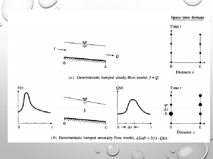
Introduction To Hydrological Models • Two classical types of hydrological models: Empirical System f(randomness, space, time) OUTPUT Deterministic Lumped conceptual Distributed physical based Steady flow Unsteady flow Time Independent Space Independent Time Correlated Stochastic INPUT Time Independent Space correlated Time Correlated

Deterministic Hydrological Models • Permit only one outcome from a simulation with one set of inputs and parameter values. • Deterministic models use physical laws (such mass and momentum conservation). • Deterministic models can be either physically based (e. g. a model based on Saint-Venant equations for flood routing) and empirical (e. g. a rating curve used as a deterministic model for predicting a sediment load from water levels). • The three main groups of deterministic models: ü Empirical models (black box) ü Lumped conceptual models (grey box) ü Distributed process (physically) description based models (white box)
 Models •")
Empirical (Black Box) Models •

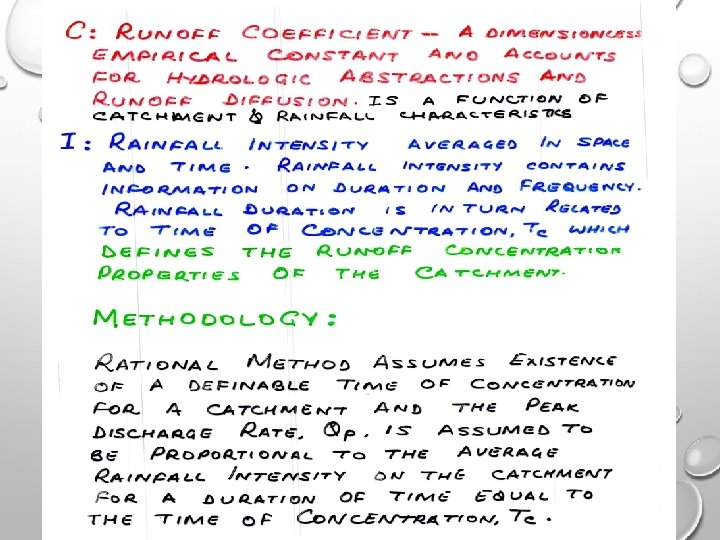
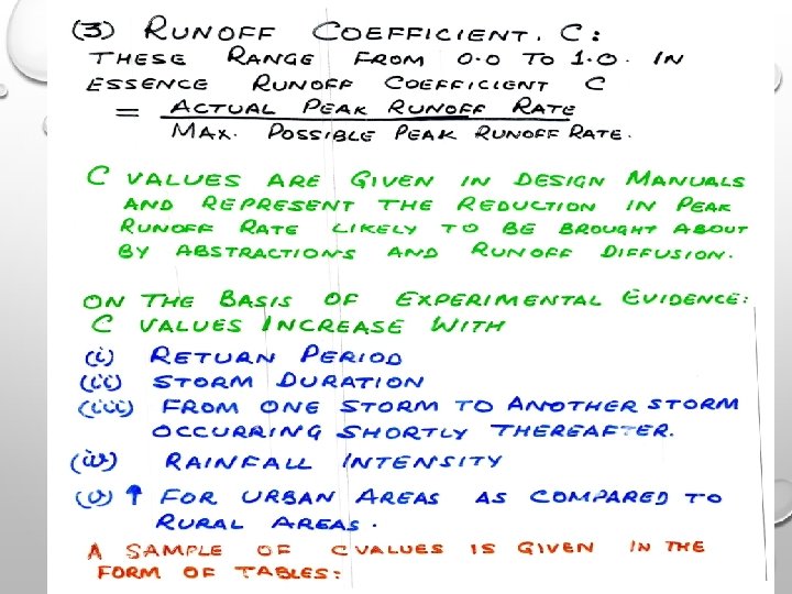
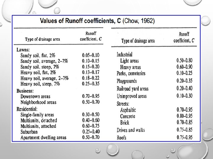
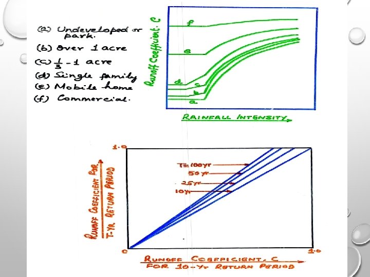
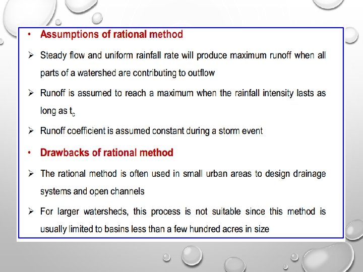
• The model reflects the way in which discharges are expected to increase with area, land use and rainfall intensity in a rational way. • The scaling parameter C reflects the fact that not all the rainfall becomes discharge. • In addition, the constant C is required to take account of the nonlinear relationship between antecedent conditions and the profile of storm rainfall and the resulting runoff production. • Thus, C is not a constant parameter, but varies from storm to storm on the same catchment, and from catchment to catchment for similar storms.

Lumped Conceptual Models • Treat the catchment as a single unit, with state variables that represent average values over the catchment area, such as storage in the saturated zone. • Description of the hydrological processes cannot be based directly on the equations that are supposed to be valid for the individual soil columns. • Hence, the equations are semi-empirical, but still with a physical basis. • Therefore, the model parameters cannot usually be assessed from field data alone, but have to be obtained through the help of calibration. • Treat precipitation input as uniform over a watershed and ignore the internal spatial variation of watershed flow.

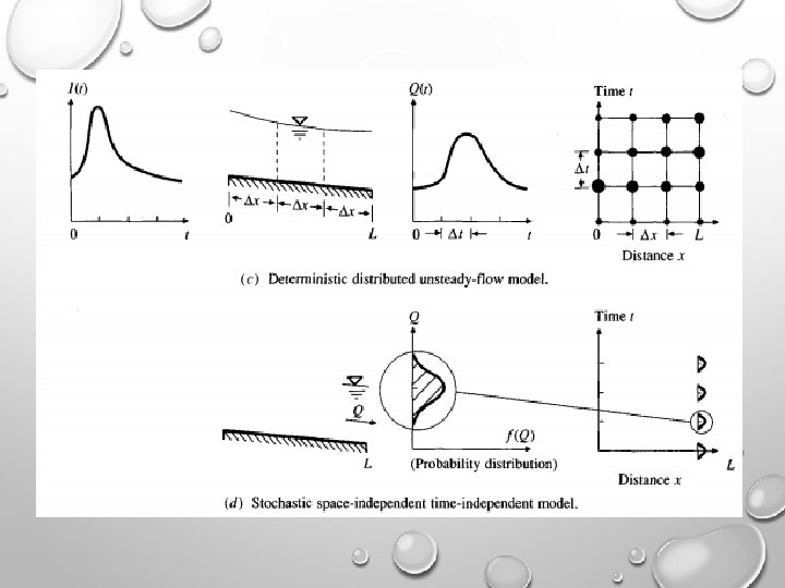
Distributed Physical Based Models • Produce models based on the governing equations describing all the surface and subsurface flow processes in the catchment. • Distributed models have the possibility of defining parameter values for every element in the solution mesh. • They give a detailed and potentially more correct description of the hydrological processes in the catchment than do the other model types. • The process equations require many different parameters to be specified for each element and made the calibration difficult in comparison with the observed responses of the catchment.

• The distributed process description based models can in principle be applied to almost any kind of hydrological problem. • Changes in land use, such as deforestation or urbanization often affect only part of a catchment area. • With a distributed model it is possible to examine the effects of such land use changes. • Considers hydrological processes taking place at various point in space and defines the model variables as a function of space dimensions.

Stochastic Time Series Models • Stochastic models allow for some randomness or uncertainty in the possible outcomes due to uncertainty in input variables, boundary conditions or model parameters. • Traditionally, a stochastic model is derived from a time series analysis of the historical record. • Used for the generation of long hypothetical sequences of events with the same statistical properties as the historical record. • In this technique several synthetic series with identical statistical properties are generated.

Stochastic Time Series Models • These generated sequences of data can then be used in the analysis of design variables and their uncertainties, for example, when estimating reservoir storage requirements. • Do not consider errors in model outcomes explicitly • We consider the hydrological variable as one for which we cannot know exact value (random variable), but for which we can calculate the probability distribution. • Model that provide probability distributions of target variables instead of single values are called stochastic models.

• In Deterministic every set of variable states is uniquely determined by parameters in the model and by sets of previous states of these variables. • Therefore, deterministic models perform the same way for a given set of initial conditions. • In a stochastic model, randomness is present, and variable states are not described by unique values, but rather by probability distributions.

• Although all hydrological phenomena involve some randomness, the resulted variability in the output may be quite small when compared to the variability resulting from known factors. In such cases, a deterministic model is appropriate • If the random variation is large, a stochastic models is more suitable, b/c the actual output could be quite different • Deterministic models of daily evaporation at a given location can be developed using energy supply and vapor transplant data • But such data cannot be used to make reliable models of daily precipitation at that location b/c precipitation is largely random. • Consequently, most daily precipitation models are stochastic.

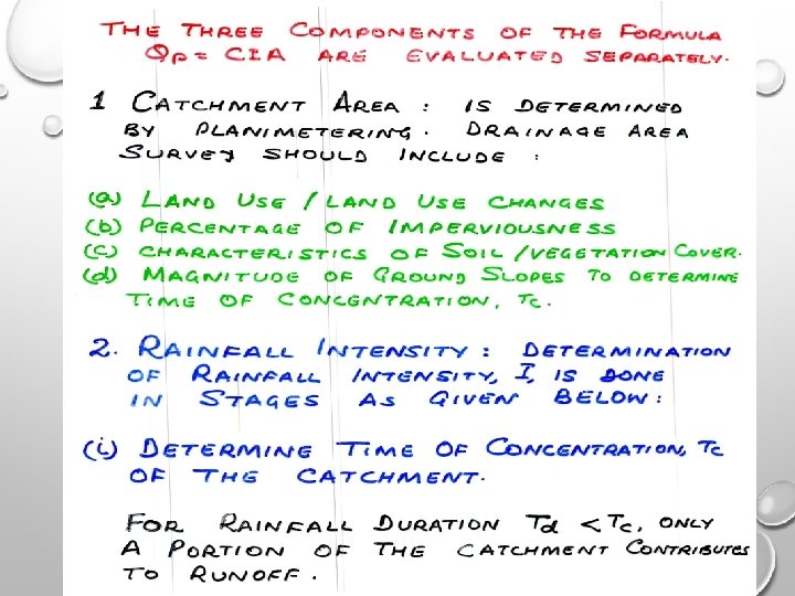
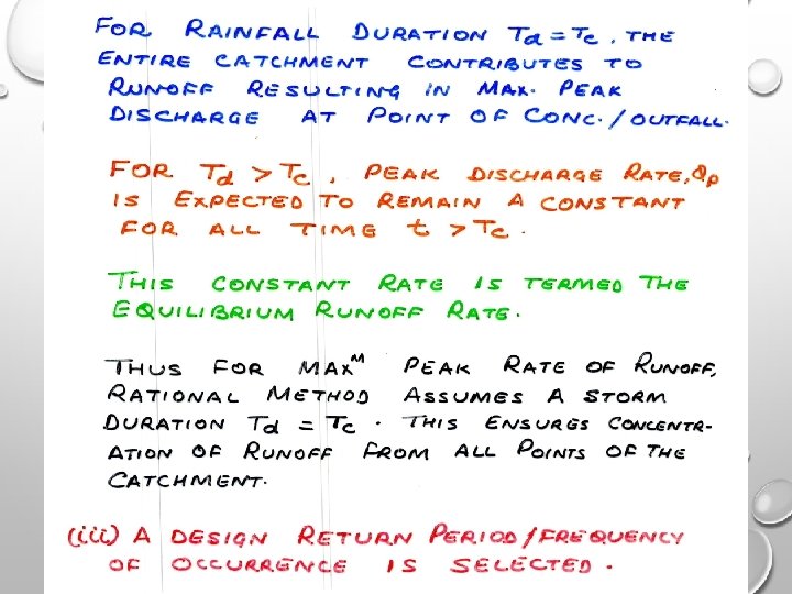
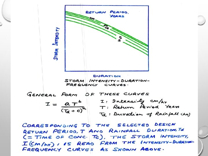
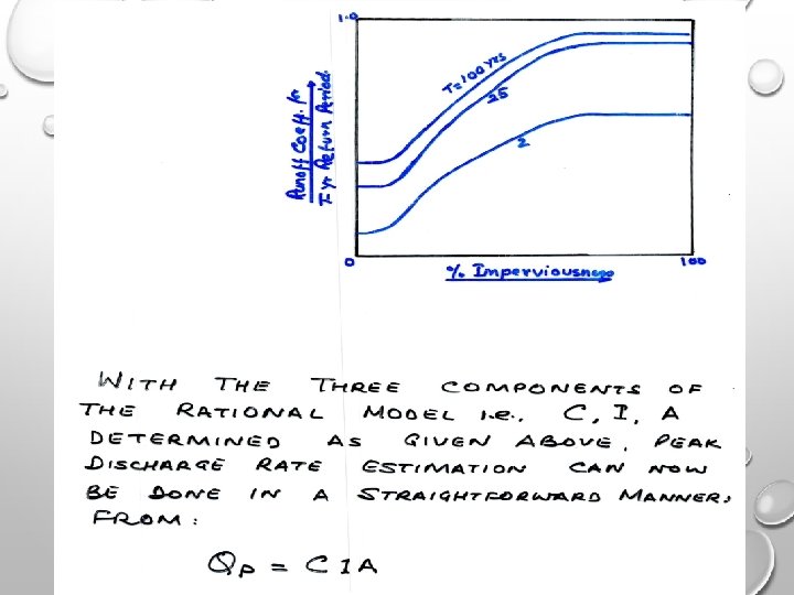
Rational Method

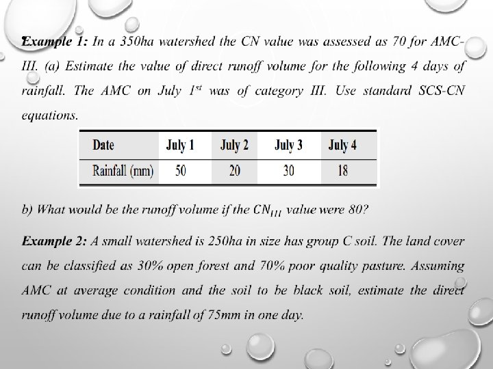
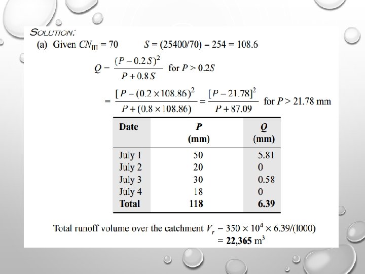
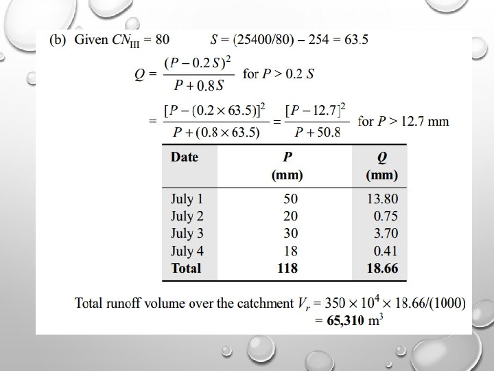
Example 1: An urban catchment has an area of 85 ha. The slope of the catchment is 0. 006 and the maximum of travel of water is 950 m. The maximum depth of rainfall with a 25 -year return period is as follows. If the culvert for drainage at the outlet of this area is to be designed for a return period of 25 years, estimate the required peak flow rate, by assuming the coefficient as 0. 3.
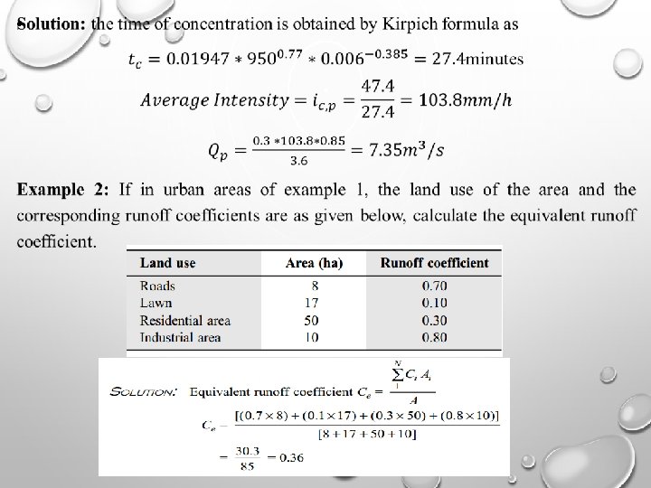

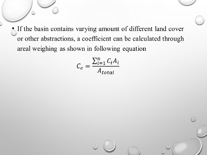
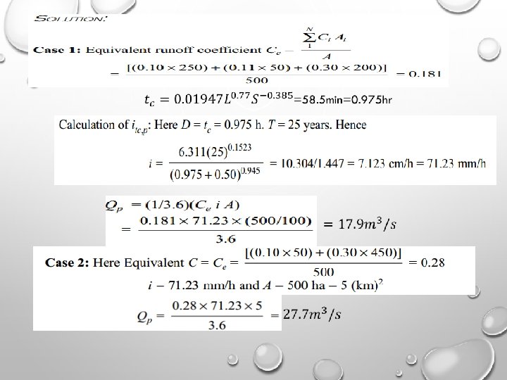
Example 3: A 500 ha watershed has the land use/ cover and the corresponding runoff coefficient as given below:

SCS Curve Number Method •
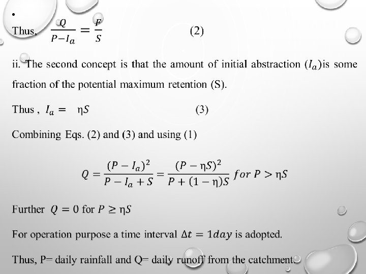
: The parameter S representing the potential maximum retention depends")
• CURVE NUMBER (CN): The parameter S representing the potential maximum retention depends upon the soil-vegetation-landuse complex of the catchment and also upon the antecedent moisture condition in the catchment just prior to the commencement of the rainfall event. • For convenience in practical application the soil conservation services (SCS) of USA has expressed S (in mm) in terms of a dimensionless parameter CN (Curve Number) as

• SOILS: In the determination of CN, the hydrological soil classification adopted. • Here, soils are classified into four classes: • Group-A: (Low Runoff Potential) • Group-B: (Moderately Low Runoff Potential) • Group-C: (Moderately High Runoff Potential) • Group-D: (High Runoff Potential) Antecedent moisture condition (AMC): Refers to the moisture content present in the soil at the beginning of the rainfall-runoff event under consideration It is well known that initial abstraction three levels of AMC are recognized by SCS as follows: AMC-I: Soils are dry but not wilting point. Satisfactory cultivation has taken place. AMC-II: Average conditions AMC-III: sufficient rainfall has occurred within the immediate past 5 days. Saturated soil conditions prevail.
 for determining the value of CN")
Antecedent moisture conditions (AMC) for determining the value of CN
 for hydrological soil cover complexes under AMC-II conditions")
Run off curve numbers (CNII) for hydrological soil cover complexes under AMC-II conditions

Solution Example-2 Referring to the table for C-group soil.

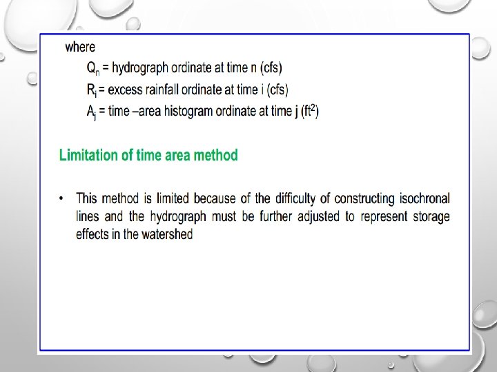
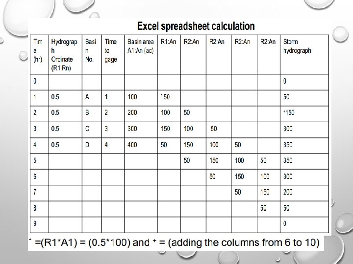
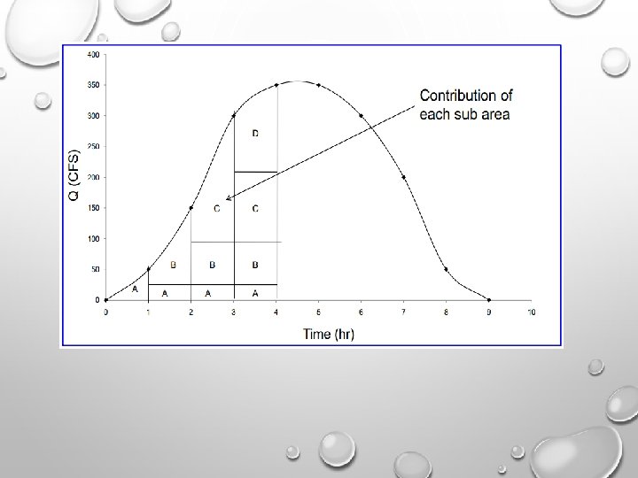
TIME-AREA METHOD
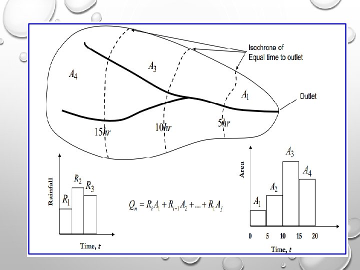

EXAMPLE PROBLEM
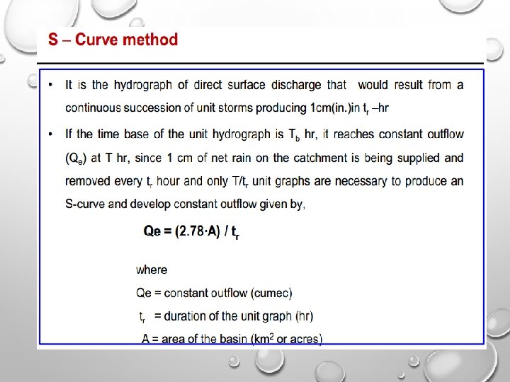
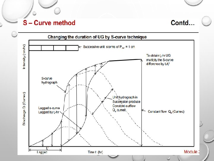
 • Defined as the hydrograph produced by unit depth of excess")
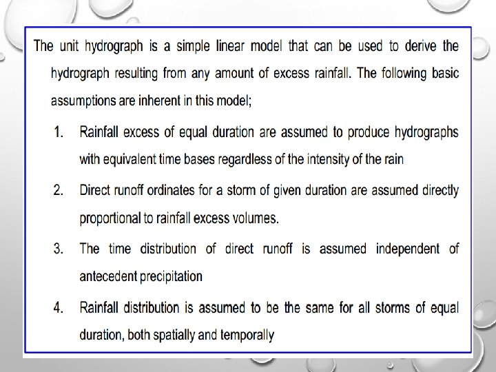
UNIT HYDROGRAPH (UH) • Defined as the hydrograph produced by unit depth of excess rainfall uniformly distributed over the entire catchment and lasting a specified duration T hrs. • The unit hydrograph is therefore called the T hr. unit hydrograph. • The unit depth refers to a fixed values and generally a depth of 1 cm or 1 inch is taken as the unit depth.

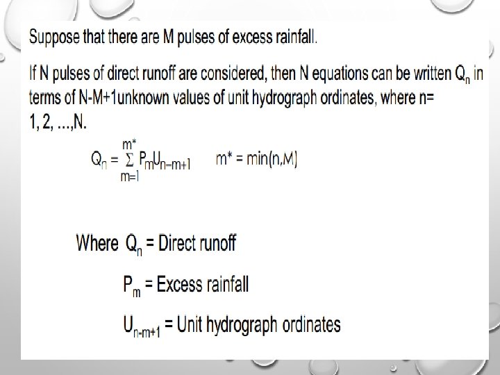
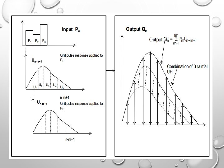
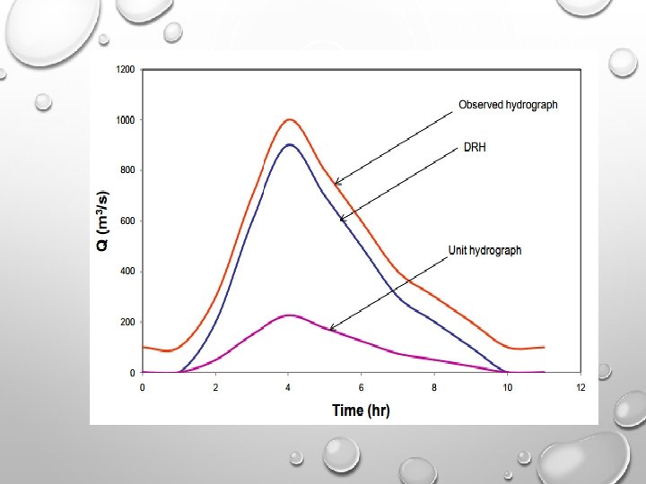
• Unit hydrograph represents the transformation of a unit depth of rainfall excess of duration T hr. into a unit depth of direct runoff and hence is a function of catchment characteristics as well as the duration of excess rain. • The resulting storm from the complex storm is divided into sub storms of equal duration and constant intensity. • After defining the effective rain from the individual storm and computing the direct runoff hydrograph, the composite DRH is obtained. • At various time intervals 1 D, 2 D, 3 D, … from the start of the ERH, let the ordinates of the unit hydrograph be U 1, U 2, U 3, … and the ordinates of the composite DRH be Q 1, Q 2, Q 3, …. Then;

1
 Number of non-zeros UH ordinates are=5 (m) Number of")
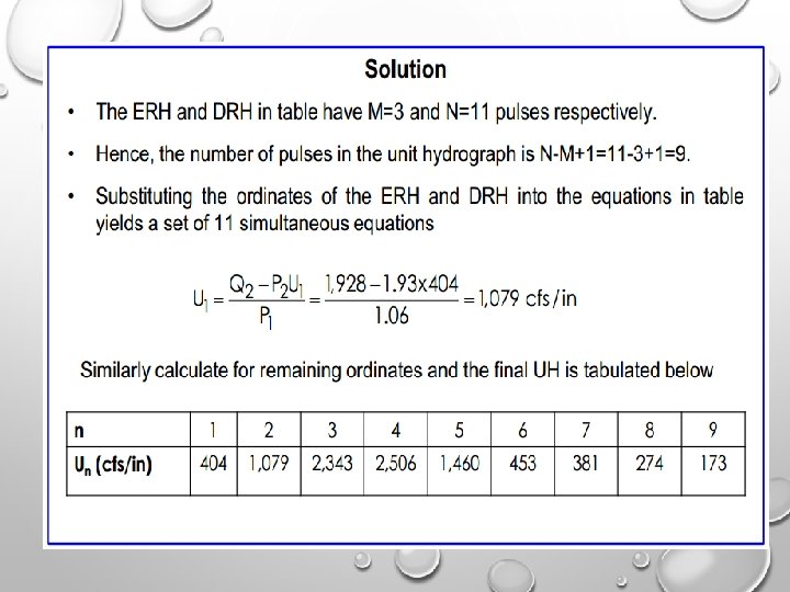
If Number of Rainfall ordinates=3(r) Number of non-zeros UH ordinates are=5 (m) Number of non-zeros DRH ordinates=7 (n) The following relationship holds n=m+r-1

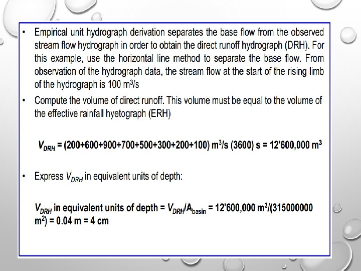
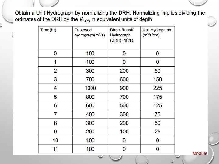
DERIVATION OF UH : GAUGED WATERSHED

RULES TO BE OBSERVED IN DEVELOPING UH FROM GAGED WATERSHEDS

ESSENTIAL STEPS FOR DEVELOPING UH FROM SINGLE STORM HYDROGRAPH

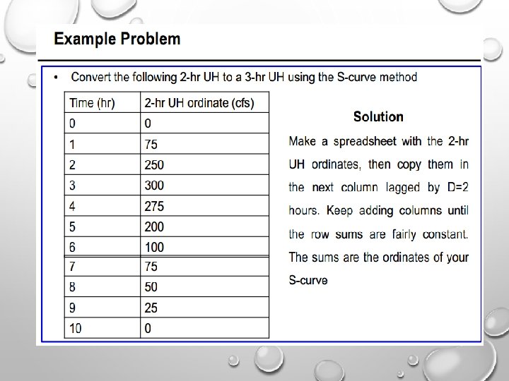
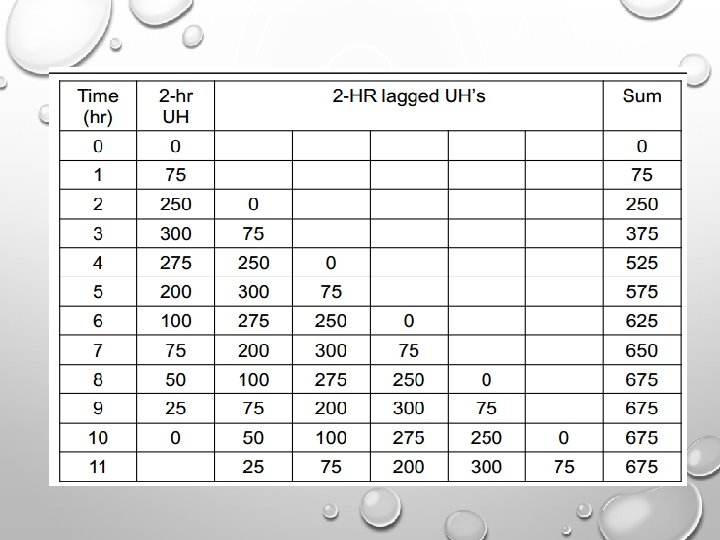
EXAMPLE PROBLEM

EXAMPLE PROBLEM
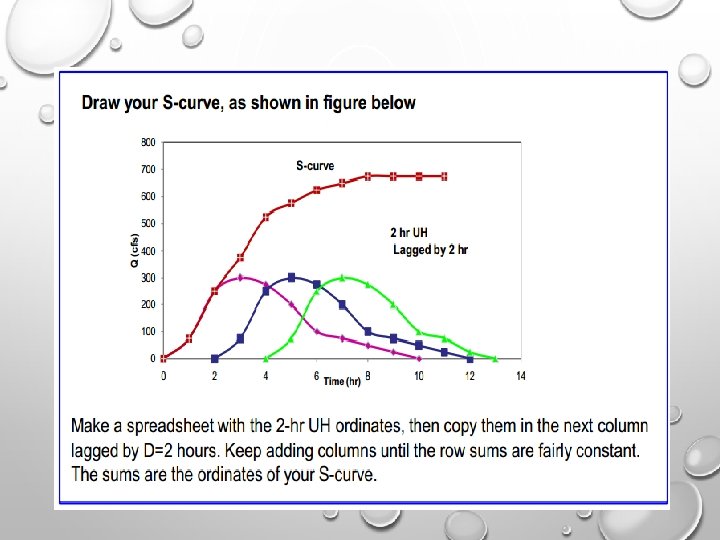
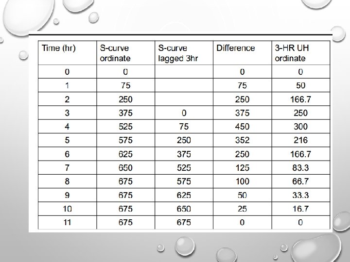

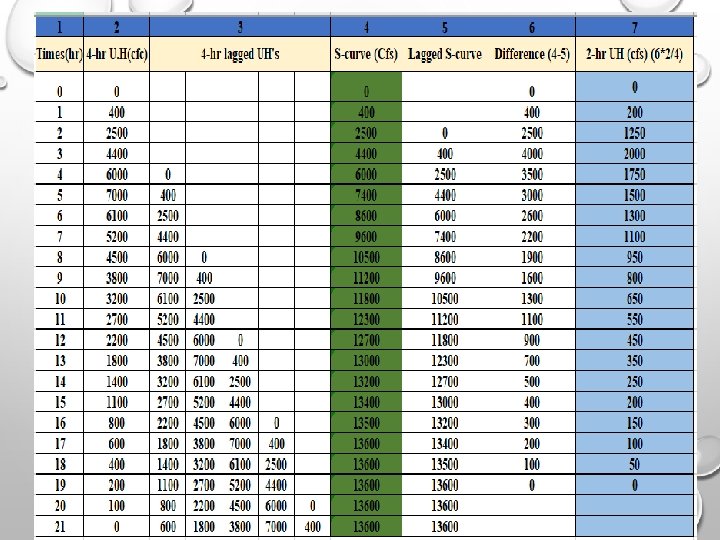
Example: Given below is the 4 -hr U. H for a basin of 84 sq. Mile. Derive S-curve and find the 2 -hr unit hydrograph. •

Example: The Ordinates Of 3 -hr U H Are Given Below: Determine the resulting flood hydrograph from the following effective rainfall Hyetograph (ERH). Assume Constant base flow of 300 cfs.

SOLUTION

QUESTIONS?
- Slides: 79