CHAPTER III LINEAR ALGEBRAIC EQUATIONS ELIAS Y 3

CHAPTER III LINEAR ALGEBRAIC EQUATIONS ELIAS Y.

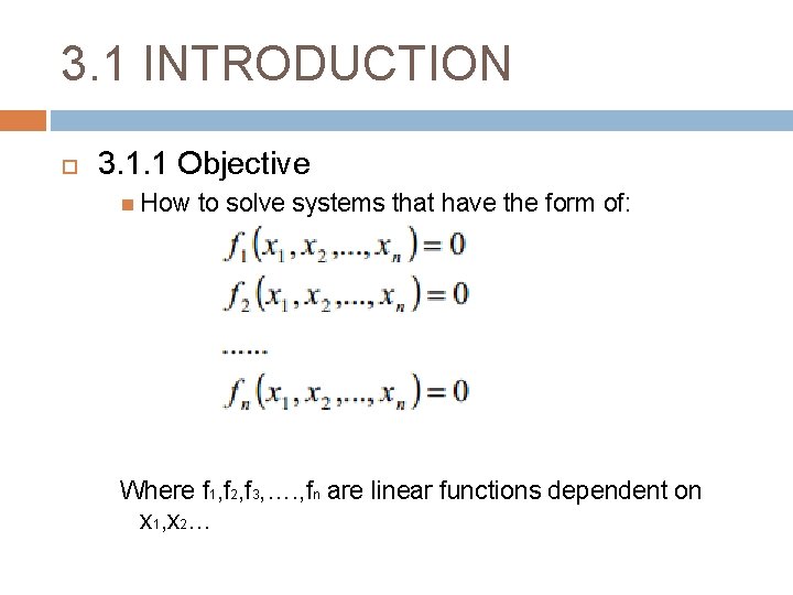
3. 1 INTRODUCTION 3. 1. 1 Objective How to solve systems that have the form of: Where f 1, f 2, f 3, …. , fn are linear functions dependent on x 1, x 2…

3. 1. 2 Contents Graphical Method Cramer’s rule Elimination Naïve Gauss Elimination Gauss-Jordan Elimination LU-Decomposition Gauss-Seidel Method

3. 2 Graphical Method For a system of linear equations, representing every equation graphically i. e. � Lines for 2 variables � Planes for 3 variables � For n variables, holding m variables constants and studying behavior graphically by varying the rest of the variables(n-m <3)

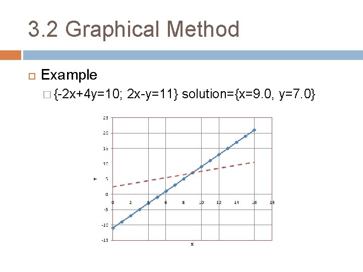
3. 2 Graphical Method Example � {-2 x+4 y=10; 2 x-y=11} solution={x=9. 0, y=7. 0}

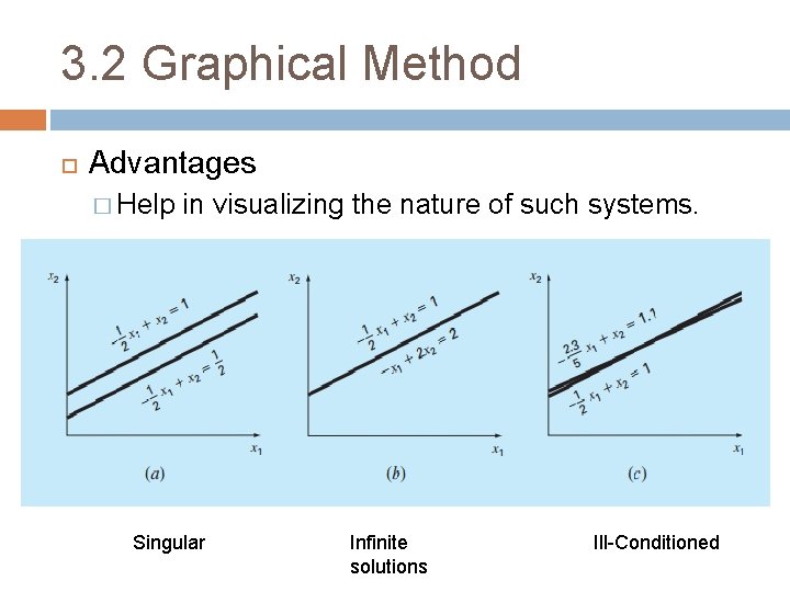
3. 2 Graphical Method Advantages � Help in visualizing the nature of such systems. Singular Infinite solutions Ill-Conditioned

3. 2 Graphical Method Disadvantages Useless for systems with rank>=3. 4 D and 5 D systems aren’t what you’d think.

3. 3 Cramer’s Rule Applicable for smaller problems [EXAMPLE] [SCILAB DEMONSTRATION]

3. 3 Cramer’s Rule [EXAMPLE] � 3 x+5 y=10 � x+2 y=5 � D=1; D 1=-5 ; D 2=5 � [solution : x=D 1/D=-5; y=D 2/D=5] [SCILAB]

3. 3 Cramer’s Rule LIMITATIONS If system is larger than rank 3, then evaluation of determinants becomes impractical.

3. 4 Elimination methods Naïve Gauss Elimination Gauss-Jordan Elimination � Pitfalls of Gauss Elimination Division by Zero Round-off Errors Ill-Conditioned systems Singular systems

3. 4. 1 Naïve Gaussian Elimination until Upper triangular matrix forms [EXAMPLE][MAXIMA demo]

3. 4. 1 Naïve Gaussian Elimination [SCILAB] (matrices and the “inv” function) >>>a=[1 2 3; -3 1 5; 2 4 -1]; >>>b=[3; -2; -1]; >>>x=inv(a)*b >>>2. -1. 1.

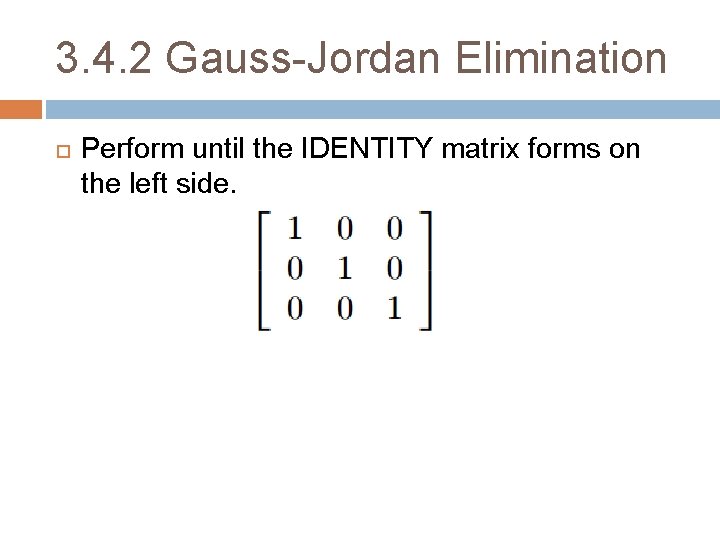
3. 4. 2 Gauss-Jordan Elimination Perform until the IDENTITY matrix forms on the left side.

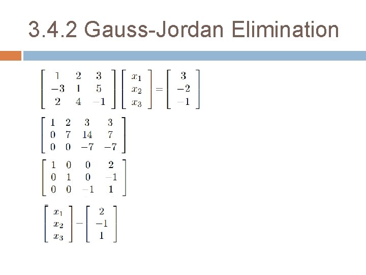
3. 4. 2 Gauss-Jordan Elimination

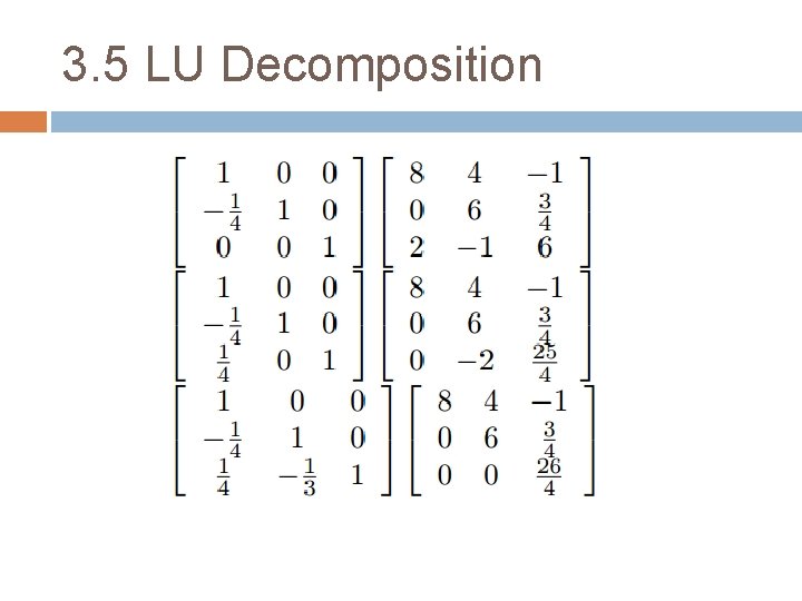
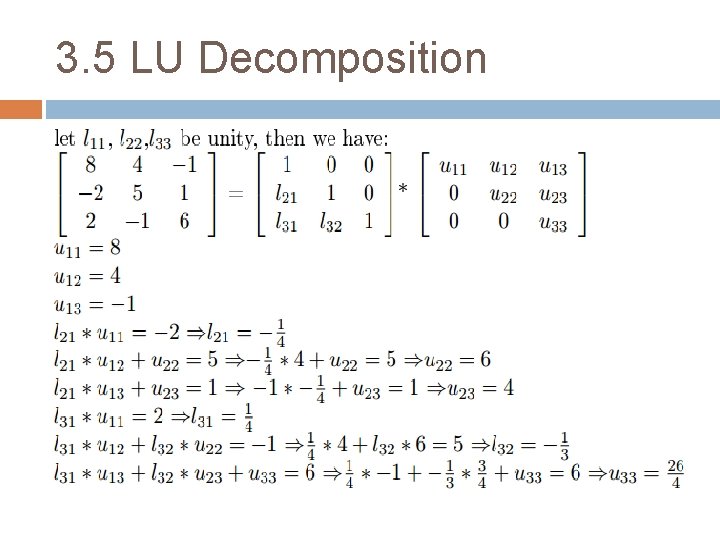
3. 5 LU Decomposition STEPS: 1. Initial : [A]{X}={B} 2. Decompose [A] into [U] and [L] 3. Construct new sets of systems: [L]{D}={B}……. (1) [U]{x}={D}……. (2) 4. Solve (1) and get {D} 5. Use {D} from step 4 to solve (2) and get {x}

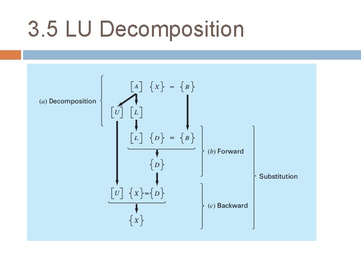
3. 5 LU Decomposition

3. 5 LU Decomposition [EXAMPLE] Step 1: Decomposition

3. 5 LU Decomposition

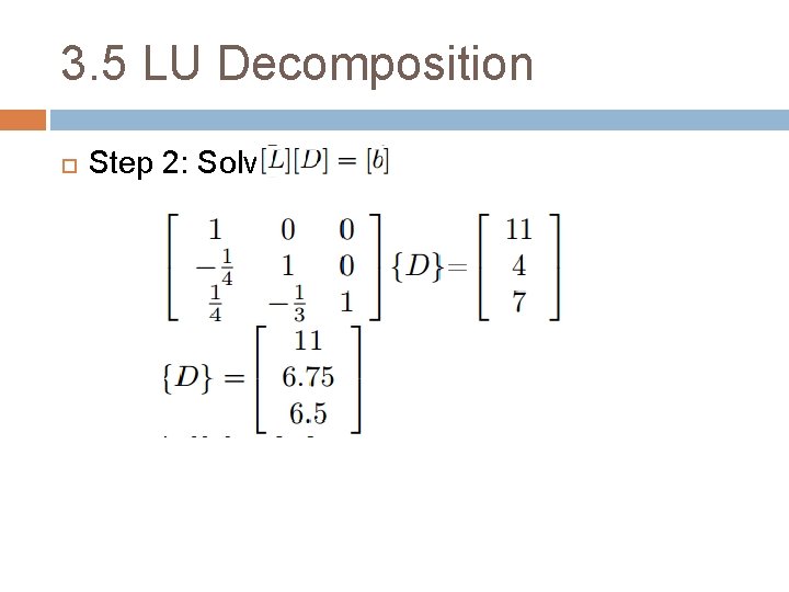
3. 5 LU Decomposition Step 2: Solve

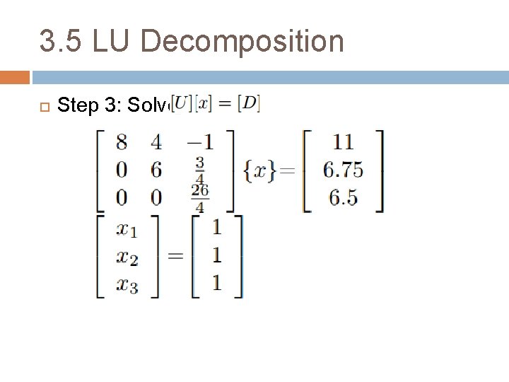
3. 5 LU Decomposition Step 3: Solve

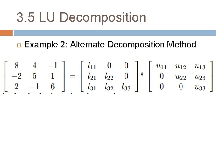
3. 5 LU Decomposition Example 2: Alternate Decomposition Method

3. 5 LU Decomposition

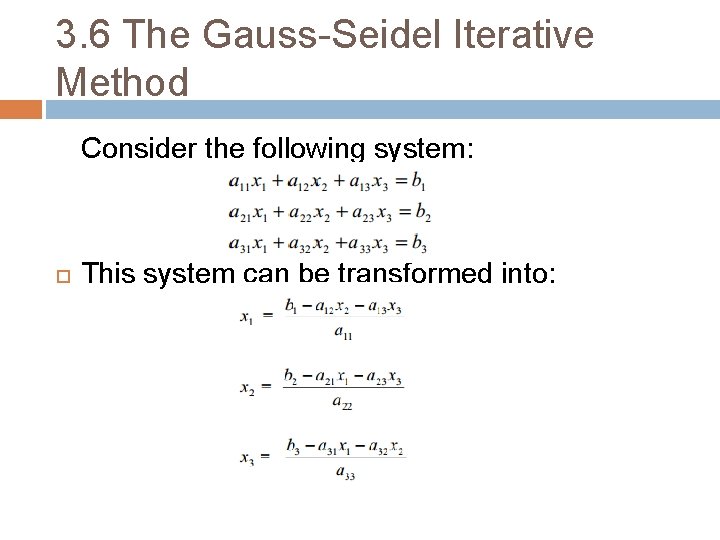
3. 6 The Gauss-Seidel Iterative Method Consider the following system: This system can be transformed into:

3. 6 The Gauss-Seidel Iterative Method Steps: 1. Assume initial guesses of x 2, x 3…. xn=selected values(usually zero) 2. Compute x 1 3. Using the result from (2) and initial guesses from step (1), Compute x 2, x 3, x 4…. , xn 4. Using newly computed values of x 2, x 3, x 4…xn compute x 1. 5. DO until convergence

3. 6 The Gauss-Seidel Iterative Method [Example][FORTRAN Demo]

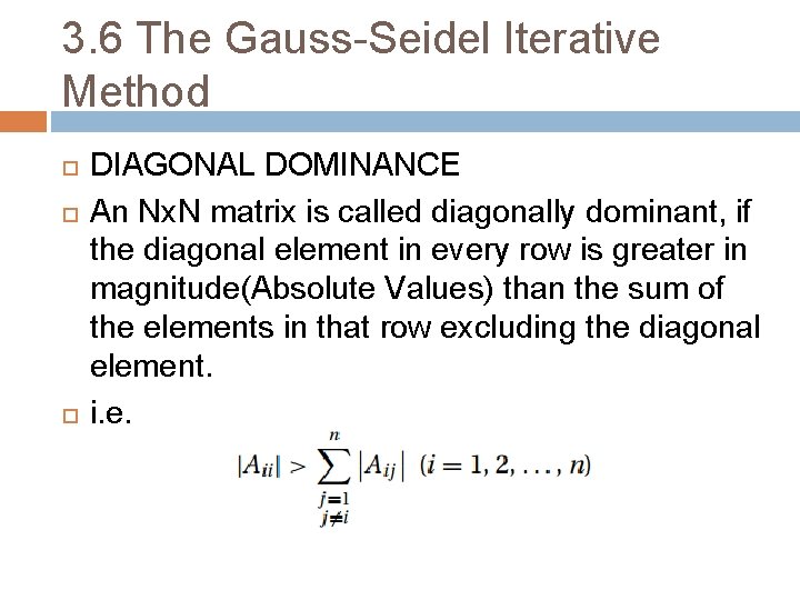
3. 6 The Gauss-Seidel Iterative Method DIAGONAL DOMINANCE An Nx. N matrix is called diagonally dominant, if the diagonal element in every row is greater in magnitude(Absolute Values) than the sum of the elements in that row excluding the diagonal element. i. e.

3. 6 The Gauss-Seidel Iterative Method [Example] � The matrix is not diagonally dominant. CHECK: row 1: |-2|<|4|+|-1| row 2: |-1|<|1|+|3| row 3: |1| < |4|+|-2|

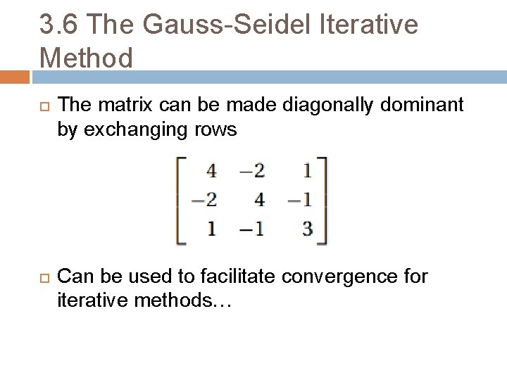
3. 6 The Gauss-Seidel Iterative Method The matrix can be made diagonally dominant by exchanging rows Can be used to facilitate convergence for iterative methods…

3. 7 The Conjugate Gradient Method [READING ASSIGNMENT]

ANY QUESTIONS ?