Chapter II Basics from probability theory and statistics

Chapter II: Basics from probability theory and statistics Information Retrieval & Data Mining Universität des Saarlandes, Saarbrücken Winter Semester 2011/12

Chapter II: Basics from Probability Theory and Statistics* II. 1 Probability Theory Events, Probabilities, Random Variables, Distributions, Moment. Generating Functions, Deviation Bounds, Limit Theorems Basics from Information Theory II. 2 Statistical Inference: Sampling and Estimation Moment Estimation, Confidence Intervals Parameter Estimation, Maximum Likelihood, EM Iteration II. 3 Statistical Inference: Hypothesis Testing and Regression Statistical Tests, p-Values, Chi-Square Test Linear and Logistic Regression *mostly following L. Wasserman, with additions from other sources IR&DM, WS'11/12 October 20, 2011 II. 2

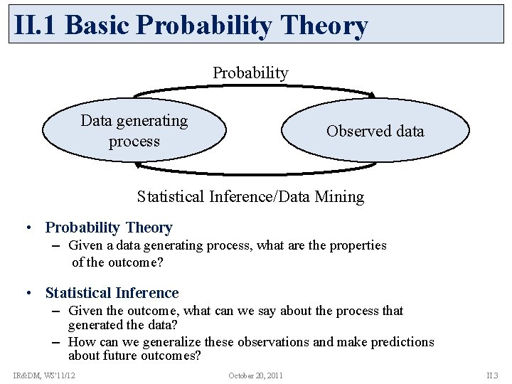
II. 1 Basic Probability Theory Probability Data generating process Observed data Statistical Inference/Data Mining • Probability Theory – Given a data generating process, what are the properties of the outcome? • Statistical Inference – Given the outcome, what can we say about the process that generated the data? – How can we generalize these observations and make predictions about future outcomes? IR&DM, WS'11/12 October 20, 2011 II. 3

Sample Spaces and Events • A sample space is a set of all possible outcomes of an experiment. (Elements e in are called sample outcomes or realizations. ) • Subsets E of are called events. Example 1: – If we toss a coin twice, then = {HH, HT, TH, TT}. – The event that the first toss is heads is A = {HH, HT}. Example 2: – Suppose we want to measure the temperature in a room. – Let = R = {-∞, ∞}, i. e. , the set of the real numbers. – The event that the temperature is between 0 and 23 degrees is A = [0, 23]. IR&DM, WS'11/12 October 20, 2011 II. 4

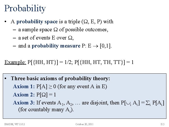
Probability • A probability space is a triple ( , E, P) with – a sample space of possible outcomes, – a set of events E over , – and a probability measure P: E [0, 1]. Example: P[{HH, HT}] = 1/2; P[{HH, HT, TH, TT}] = 1 • Three basic axioms of probability theory: Axiom 1: P[A] ≥ 0 (for any event A in E) Axiom 2: P[ ] = 1 Axiom 3: If events A 1, A 2, … are disjoint, then P[ i Ai] = i P[Ai] (for countably many Ai). IR&DM, WS'11/12 October 20, 2011 II. 5

Probability More properties (derived from axioms) P[ ] = 0 (null/impossible event) P[ ] = 1 (true/certain event, actually not derived but 2 nd axiom) 0 ≤ P[A] ≤ 1 If A B then P[A] ≤ P[B] P[A] + P[ A] = 1 P[A B] = P[A] + P[B] – P[A B] (inclusion-exclusion principle) Notes: – E is closed under , , and – with a countable number of operands (with finite , usually E=2 ). – It is not always possible to assign a probability to every event in E if the sample space is large. Instead one may assign probabilities to a limited class of sets in E. IR&DM, WS'11/12 October 20, 2011 II. 6

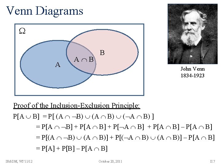
Venn Diagrams A A B B John Venn 1834 -1923 Proof of the Inclusion-Exclusion Principle: P[A B] = P[ (A B) ( A B) ] = P[A B] + P[A B] – P[A B] = P[(A B) (A B)] + P[( A B) (A B)] – P[A B] = P[A] + P[B] – P[A B] IR&DM, WS'11/12 October 20, 2011 II. 7

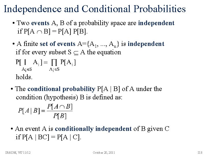
Independence and Conditional Probabilities • Two events A, B of a probability space are independent if P[A B] = P[A] P[B]. • A finite set of events A={A 1, . . . , An} is independent if for every subset S A the equation holds. • The conditional probability P[A | B] of A under the condition (hypothesis) B is defined as: • An event A is conditionally independent of B given C if P[A | BC] = P[A | C]. IR&DM, WS'11/12 October 20, 2011 II. 8

Independence vs. Disjointness Set-Complement P[⌐A] = 1 – P[A] Independence P[A B] = P[A] P[B] P[A B] = 1 – (1 – P[A])(1 – P[B]) Disjointness P[A B] = 0 P[A B] = P[A] + P[B] Identity IR&DM, WS'11/12 P[A] = P[B] = P[A B] October 20, 2011 II. 9

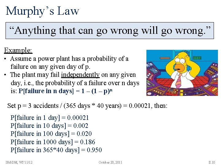
Murphy’s Law “Anything that can go wrong will go wrong. ” Example: • Assume a power plant has a probability of a failure on any given day of p. • The plant may fail independently on any given day, i. e. , the probability of a failure over n days is: P[failure in n days] = 1 – (1 – p)n Set p = 3 accidents / (365 days * 40 years) = 0. 00021, then: P[failure in 1 day] = 0. 00021 P[failure in 10 days] = 0. 002 P[failure in 100 days] = 0. 020 P[failure in 1000 days] = 0. 186 P[failure in 365*40 days] = 0. 950 IR&DM, WS'11/12 October 20, 2011 II. 10

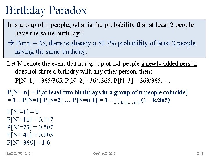
Birthday Paradox In a group of n people, what is the probability that at least 2 people have the same birthday? For n = 23, there is already a 50. 7% probability of least 2 people having the same birthday. Let N denote the event that in a group of n-1 people a newly added person does not share a birthday with any other person, then: P[N=1] = 365/365, P[N=2]= 364/365, P[N=3] = 363/365, … P[N’=n] = P[at least two birthdays in a group of n people coincide] = 1 – P[N=1] P[N=2] … P[N=n-1] = 1 – ∏ k=1, …, n-1 (1 – k/365) P[N’=1] = 0 P[N’=10] = 0. 117 P[N’=23] = 0. 507 P[N’=41] = 0. 903 P[N’=366] = 1. 0 IR&DM, WS'11/12 October 20, 2011 II. 11

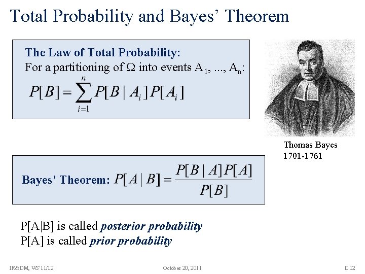
Total Probability and Bayes’ Theorem The Law of Total Probability: For a partitioning of into events A 1, . . . , An: Thomas Bayes 1701 -1761 Bayes’ Theorem: P[A|B] is called posterior probability P[A] is called prior probability IR&DM, WS'11/12 October 20, 2011 II. 12

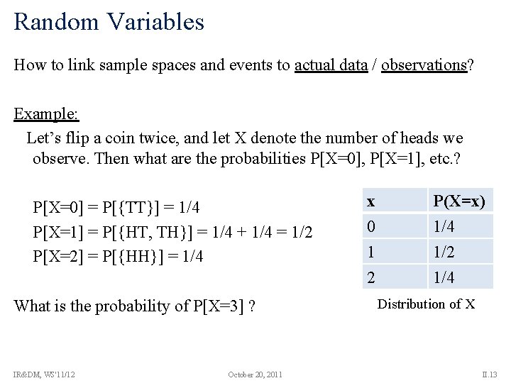
Random Variables How to link sample spaces and events to actual data / observations? Example: Let’s flip a coin twice, and let X denote the number of heads we observe. Then what are the probabilities P[X=0], P[X=1], etc. ? P[X=0] = P[{TT}] = 1/4 P[X=1] = P[{HT, TH}] = 1/4 + 1/4 = 1/2 P[X=2] = P[{HH}] = 1/4 What is the probability of P[X=3] ? IR&DM, WS'11/12 October 20, 2011 x 0 1 2 P(X=x) 1/4 1/2 1/4 Distribution of X II. 13

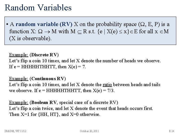
Random Variables • A random variable (RV) X on the probability space ( , E, P) is a function X: M with M R s. t. {e | X(e) x} E for all x M (X is observable). Example: (Discrete RV) Let’s flip a coin 10 times, and let X denote the number of heads we observe. If e = HHHHHTHHTT, then X(e) = 7. Example: (Continuous RV) Let’s flip a coin 10 times, and let X denote the ratio between heads and tails we observe. If e = HHHHHTHHTT, then X(e) = 7/3. Example: (Boolean RV, special case of a discrete RV) Let’s flip a coin twice, and let X denote the event that heads occurs first. Then X=1 for {HH, HT}, and X=0 otherwise. IR&DM, WS'11/12 October 20, 2011 II. 14

Distribution and Density Functions • FX: M [0, 1] with FX(x) = P[X x] is the cumulative distribution function (cdf) of X. • For a countable set M, the function f. X: M [0, 1] with f. X(x) = P[X = x] is called the probability density function (pdf) of X; in general f. X(x) is F’X(x). • For a random variable X with distribution function F, the inverse function F-1(q) : = inf{x | F(x) > q} for q [0, 1] is called quantile function of X. (the 0. 5 quantile (aka. “ 50 th percentile”) is called median) Random variables with countable M are called discrete, otherwise they are called continuous. For discrete random variables, the density function is also referred to as the probability mass function. IR&DM, WS'11/12 October 20, 2011 II. 15

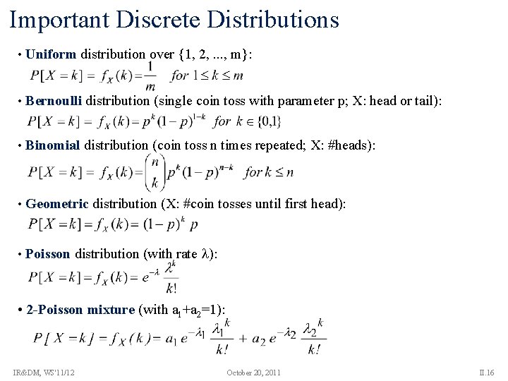
Important Discrete Distributions • Uniform distribution over {1, 2, . . . , m}: • Bernoulli distribution (single coin toss with parameter p; X: head or tail): • Binomial distribution (coin toss n times repeated; X: #heads): • Geometric distribution (X: #coin tosses until first head): • Poisson distribution (with rate ): • 2 -Poisson mixture (with a 1+a 2=1): IR&DM, WS'11/12 October 20, 2011 II. 16

Important Continuous Distributions • Uniform distribution in the interval [a, b] • Exponential distribution (e. g. time until next event of a Poisson process) with rate = lim t 0 (# events in t) / t : • Hyper-exponential distribution: • Pareto distribution: Example of a “heavy-tailed” distribution with • Logistic distribution: IR&DM, WS'11/12 October 20, 2011 II. 17

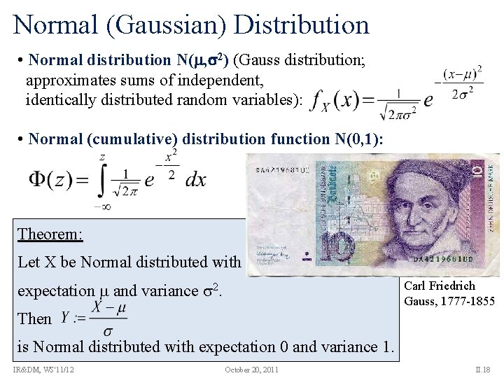
Normal (Gaussian) Distribution • Normal distribution N( , 2) (Gauss distribution; approximates sums of independent, identically distributed random variables): • Normal (cumulative) distribution function N(0, 1): Theorem: Let X be Normal distributed with Carl Friedrich Gauss, 1777 -1855 expectation and variance 2. Then is Normal distributed with expectation 0 and variance 1. IR&DM, WS'11/12 October 20, 2011 II. 18

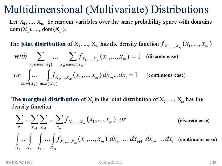
Multidimensional (Multivariate) Distributions Let X 1, . . . , Xm be random variables over the same probability space with domains dom(X 1), . . . , dom(Xm). The joint distribution of X 1, . . . , Xm has the density function (discrete case) (continuous case) The marginal distribution of Xi in the joint distribution of X 1, . . . , Xm has the density function (discrete case) (continuous case) IR&DM, WS'11/12 October 20, 2011 II. 19

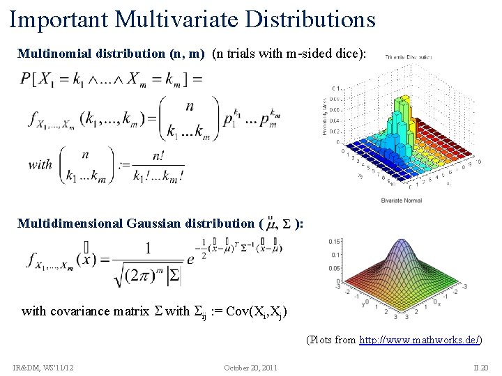
Important Multivariate Distributions Multinomial distribution (n, m) (n trials with m-sided dice): Multidimensional Gaussian distribution ( ): with covariance matrix with ij : = Cov(Xi, Xj) (Plots from http: //www. mathworks. de/) IR&DM, WS'11/12 October 20, 2011 II. 20

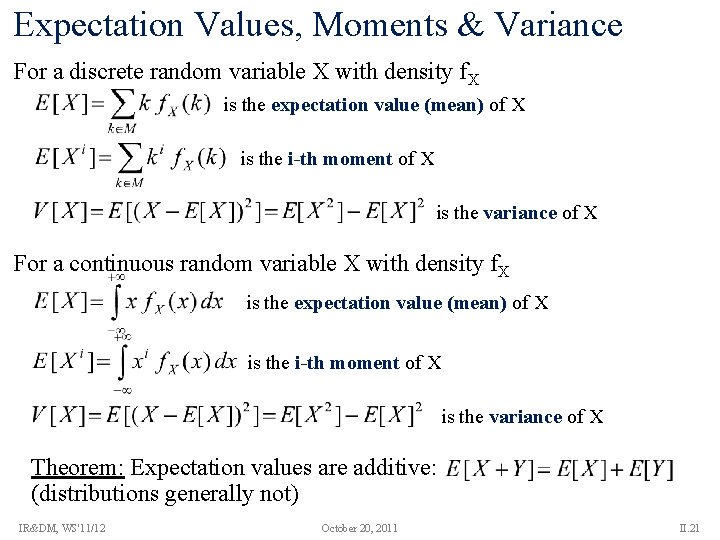
Expectation Values, Moments & Variance For a discrete random variable X with density f. X is the expectation value (mean) of X is the i-th moment of X is the variance of X For a continuous random variable X with density f. X is the expectation value (mean) of X is the i-th moment of X is the variance of X Theorem: Expectation values are additive: (distributions generally not) IR&DM, WS'11/12 October 20, 2011 II. 21

Properties of Expectation and Variance • E[a. X+b] = a. E[X]+b for constants a, b • E[X 1+X 2+. . . +Xn] = E[X 1] + E[X 2] +. . . + E[Xn] (i. e. expectation values are generally additive, but distributions are not!) • E[XY] = E[X]E[Y] if X and Y are independent • E[X 1+X 2+. . . +XN] = E[N] E[X] if X 1, X 2, . . . , XN are independent and identically distributed (iid) RVs with mean E[X] and N is a stopping-time RV • Var[a. X+b] = a 2 Var[X] for constants a, b • Var[X 1+X 2+. . . +Xn] = Var[X 1] + Var[X 2] +. . . + Var[Xn] if X 1, X 2, . . . , Xn are independent RVs • Var[X 1+X 2+. . . +XN] = E[N] Var[X] + E[X]2 Var[N] if X 1, X 2, . . . , XN are iid RVs with mean E[X] and variance Var[X] and N is a stopping-time RV IR&DM, WS'11/12 October 20, 2011 II. 22

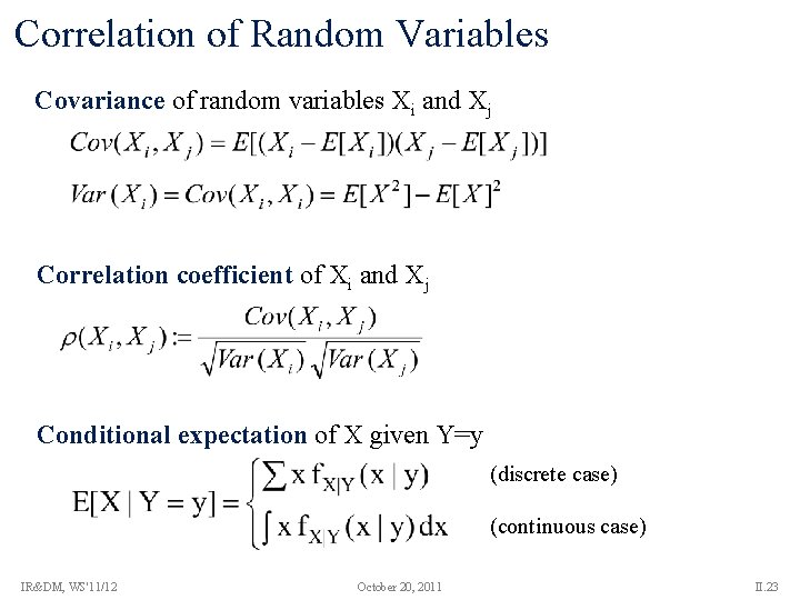
Correlation of Random Variables Covariance of random variables Xi and Xj Correlation coefficient of Xi and Xj Conditional expectation of X given Y=y (discrete case) (continuous case) IR&DM, WS'11/12 October 20, 2011 II. 23

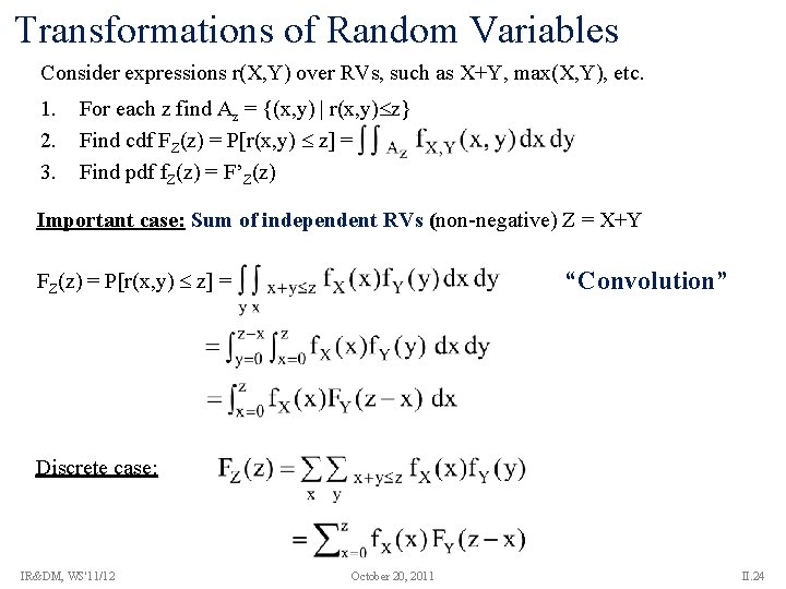
Transformations of Random Variables Consider expressions r(X, Y) over RVs, such as X+Y, max(X, Y), etc. 1. 2. 3. For each z find Az = {(x, y) | r(x, y) z} Find cdf FZ(z) = P[r(x, y) z] = Find pdf f. Z(z) = F’Z(z) Important case: Sum of independent RVs (non-negative) Z = X+Y “Convolution” FZ(z) = P[r(x, y) z] = Discrete case: IR&DM, WS'11/12 October 20, 2011 II. 24

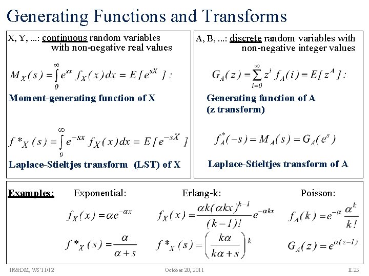
Generating Functions and Transforms X, Y, . . . : continuous random variables with non-negative real values A, B, . . . : discrete random variables with non-negative integer values Moment-generating function of X Generating function of A (z transform) Laplace-Stieltjes transform (LST) of X Laplace-Stieltjes transform of A Examples: IR&DM, WS'11/12 Exponential: Erlang-k: October 20, 2011 Poisson: II. 25

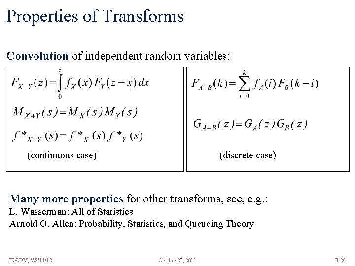
Properties of Transforms Convolution of independent random variables: (continuous case) (discrete case) Many more properties for other transforms, see, e. g. : L. Wasserman: All of Statistics Arnold O. Allen: Probability, Statistics, and Queueing Theory IR&DM, WS'11/12 October 20, 2011 II. 26

Use Case: Score prediction for fast Top-k [Theobald, Schenkel, Weikum: VLDB’ 04] Queries L 1 L 2 L 3 D 10: 0. 8 D 4: 1. 0 D 6 : 0. 9 D 7 : 0. 8 D 9 : 0. 9 D 7 : 0. 8 D 21: 0. 7 D 1: 0. 8 D 10: 0. 6 high 2 high 3 … … high 1 … D 21: 0. 6 Given: Inverted lists Li with continuous score distributions captured by independent RV’s Si Want to predict: • Consider score intervals [0, highi ] at current scan positions in Li, then fi(x) = 1/highi (assuming uniform score distributions) • Convolution S 1+S 2 is given by • But each factor is non-zero in 0 ≤ x ≤ high 1 and 0 ≤ z-x ≤ high 2 only (for high 1≤ high 2), thus D 21: 0. 3 … … IR&DM, WS'11/12 … Cumbersome amount of case differentiations October 20, 2011 II. 27

Use Case: Score prediction for fast Top-k [Theobald, Schenkel, Weikum: VLDB’ 04] Queries L 1 L 2 L 3 D 10: 0. 8 D 4: 1. 0 D 6 : 0. 9 D 7 : 0. 8 D 9 : 0. 9 D 7 : 0. 8 D 21: 0. 7 D 1: 0. 8 D 10: 0. 6 high 2 high 3 … … high 1 … D 21: 0. 6 Given: Inverted lists Li with continuous score distributions captured by independent RV’s Si Want to predict: • Instead: Consider the moment-generating function for each Si • For independent Si, the moment of the convolution over all Si is given by • Apply Chernoff-Hoeffding bound on tail distribution D 21: 0. 3 … … IR&DM, WS'11/12 … Prune D 21 if P[S 2+S 3 > δ] ≤ ε (using δ = 1. 4 -0. 7 and a small confidence threshold for ε, e. g. , ε=0. 05) October 20, 2011 II. 28

Inequalities and Tail Bounds Markov inequality: P[X t] E[X] / t for t > 0 and non-neg. RV X Chebyshev inequality: P[ |X E[X]| t] Var[X] / t 2 for t > 0 and non-neg. RV X Chernoff-Hoeffding bound: Corollary: for Bernoulli(p) iid. RVs X 1, . . . , Xn and any t > 0 Mill‘s inequality: for N(0, 1) distr. RV Z and t > 0 Cauchy-Schwarz inequality: Jensen’s inequality: E[g(X)] g(E[X]) for convex function g E[g(X)] g(E[X]) for concave function g (g is convex if for all c [0, 1] and x 1, x 2: g(cx 1 + (1 -c)x 2) cg(x 1) + (1 -c)g(x 2)) IR&DM, WS'11/12 October 20, 2011 II. 29

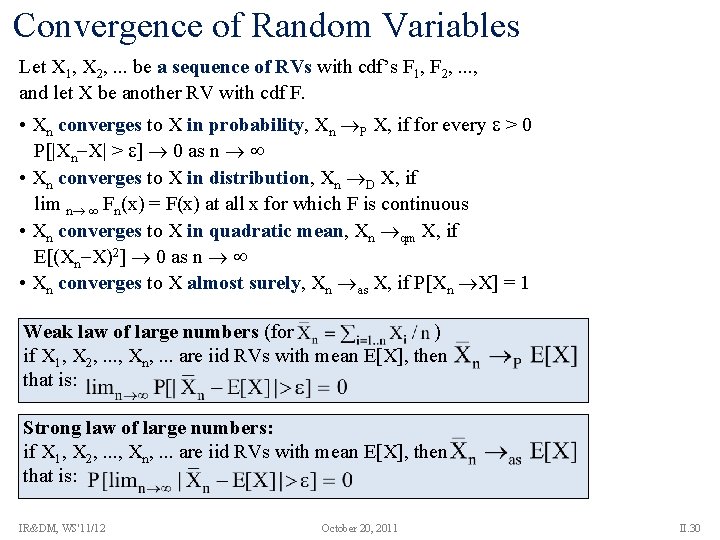
Convergence of Random Variables Let X 1, X 2, . . . be a sequence of RVs with cdf’s F 1, F 2, . . . , and let X be another RV with cdf F. • Xn converges to X in probability, Xn P X, if for every > 0 P[|Xn X| > ] 0 as n • Xn converges to X in distribution, Xn D X, if lim n Fn(x) = F(x) at all x for which F is continuous • Xn converges to X in quadratic mean, Xn qm X, if E[(Xn X)2] 0 as n • Xn converges to X almost surely, Xn as X, if P[Xn X] = 1 Weak law of large numbers (for ) if X 1, X 2, . . . , Xn, . . . are iid RVs with mean E[X], then that is: Strong law of large numbers: if X 1, X 2, . . . , Xn, . . . are iid RVs with mean E[X], then that is: IR&DM, WS'11/12 October 20, 2011 II. 30

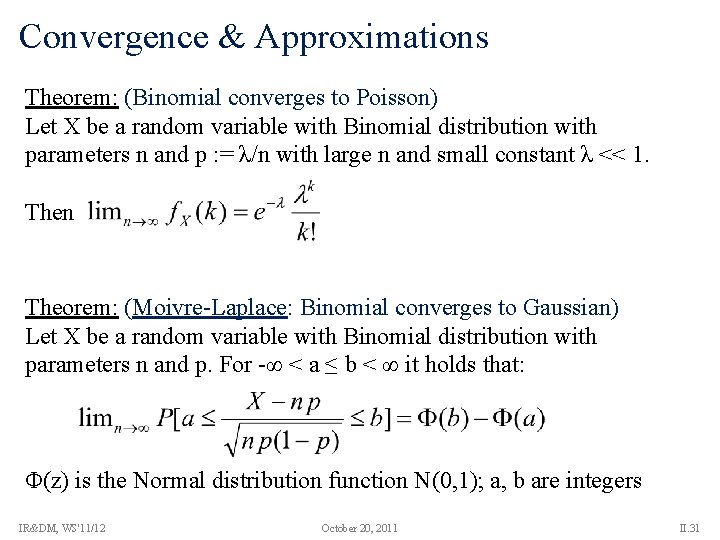
Convergence & Approximations Theorem: (Binomial converges to Poisson) Let X be a random variable with Binomial distribution with parameters n and p : = λ/n with large n and small constant λ << 1. Then Theorem: (Moivre-Laplace: Binomial converges to Gaussian) Let X be a random variable with Binomial distribution with parameters n and p. For -∞ < a ≤ b < ∞ it holds that: Φ(z) is the Normal distribution function N(0, 1); a, b are integers IR&DM, WS'11/12 October 20, 2011 II. 31

Central Limit Theorem: Let X 1, . . . , Xn be n independent, identically distributed (iid) random variables with expectation µ and variance σ2. The distribution function Fn of the random variable Zn : = X 1 +. . . + Xn converges to a Normal distribution N(nμ, nσ2) with expectation nμ and variance nσ2. That is, for -∞ < x ≤ y < ∞ it holds that: Corollary: converges to a Normal distribution N(μ, σ2/n) with expectation μ and variance σ2/n. IR&DM, WS'11/12 October 20, 2011 II. 32

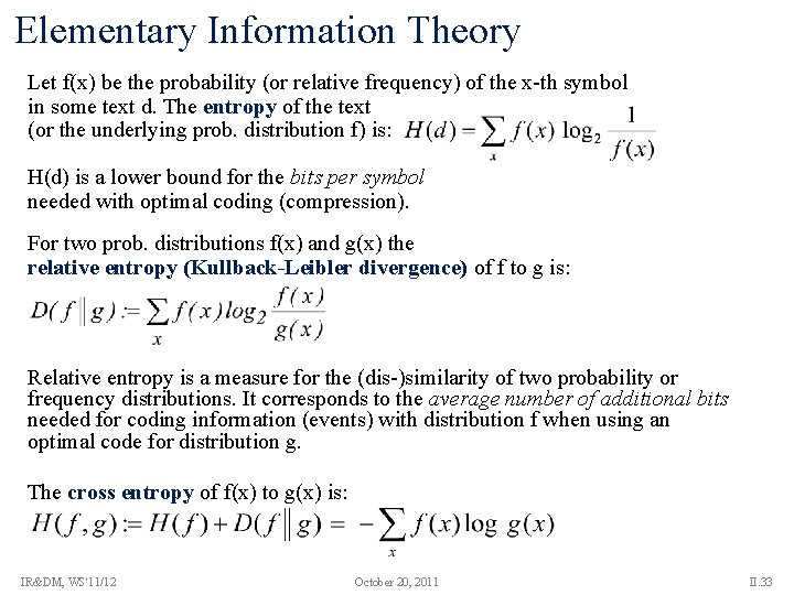
Elementary Information Theory Let f(x) be the probability (or relative frequency) of the x-th symbol in some text d. The entropy of the text (or the underlying prob. distribution f) is: H(d) is a lower bound for the bits per symbol needed with optimal coding (compression). For two prob. distributions f(x) and g(x) the relative entropy (Kullback-Leibler divergence) of f to g is: Relative entropy is a measure for the (dis-)similarity of two probability or frequency distributions. It corresponds to the average number of additional bits needed for coding information (events) with distribution f when using an optimal code for distribution g. The cross entropy of f(x) to g(x) is: IR&DM, WS'11/12 October 20, 2011 II. 33

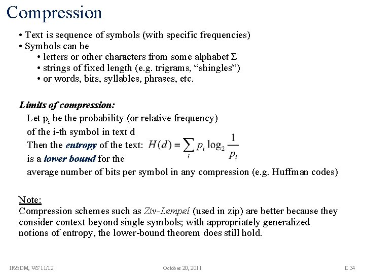
Compression • Text is sequence of symbols (with specific frequencies) • Symbols can be • letters or other characters from some alphabet Σ • strings of fixed length (e. g. trigrams, “shingles”) • or words, bits, syllables, phrases, etc. Limits of compression: Let pi be the probability (or relative frequency) of the i-th symbol in text d Then the entropy of the text: is a lower bound for the average number of bits per symbol in any compression (e. g. Huffman codes) Note: Compression schemes such as Ziv-Lempel (used in zip) are better because they consider context beyond single symbols; with appropriately generalized notions of entropy, the lower-bound theorem does still hold. IR&DM, WS'11/12 October 20, 2011 II. 34

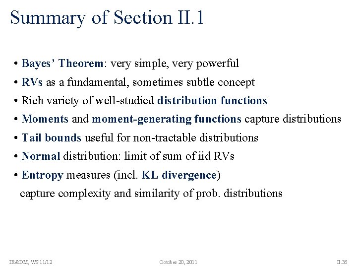
Summary of Section II. 1 • Bayes’ Theorem: very simple, very powerful • RVs as a fundamental, sometimes subtle concept • Rich variety of well-studied distribution functions • Moments and moment-generating functions capture distributions • Tail bounds useful for non-tractable distributions • Normal distribution: limit of sum of iid RVs • Entropy measures (incl. KL divergence) capture complexity and similarity of prob. distributions IR&DM, WS'11/12 October 20, 2011 II. 35

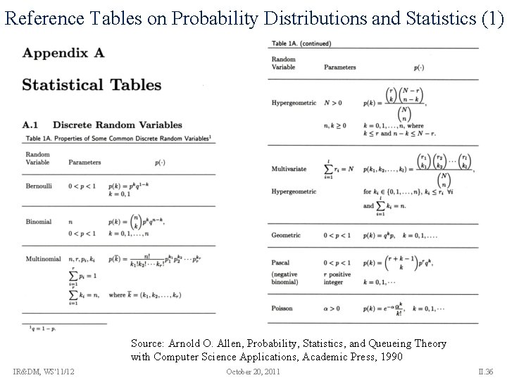
Reference Tables on Probability Distributions and Statistics (1) Source: Arnold O. Allen, Probability, Statistics, and Queueing Theory with Computer Science Applications, Academic Press, 1990 IR&DM, WS'11/12 October 20, 2011 II. 36

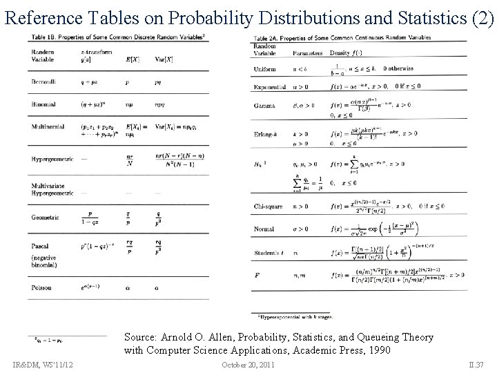
Reference Tables on Probability Distributions and Statistics (2) Source: Arnold O. Allen, Probability, Statistics, and Queueing Theory with Computer Science Applications, Academic Press, 1990 IR&DM, WS'11/12 October 20, 2011 II. 37

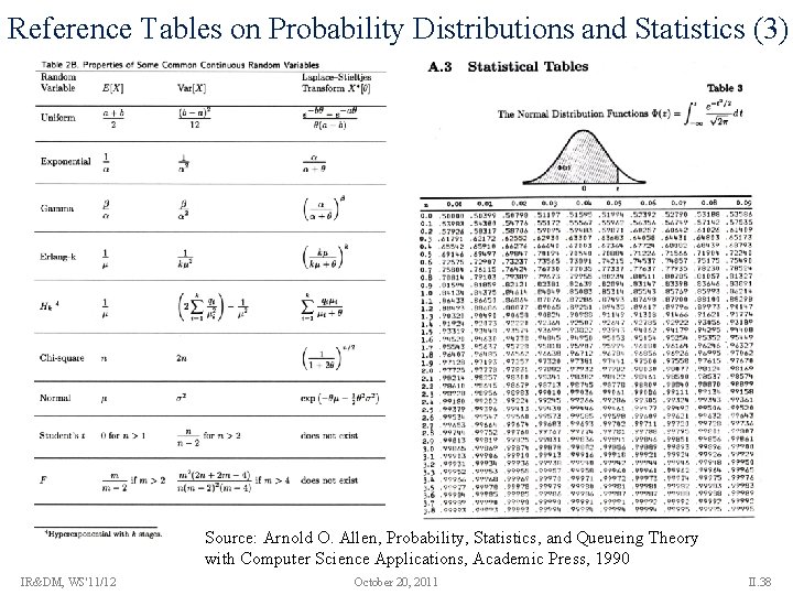
Reference Tables on Probability Distributions and Statistics (3) Source: Arnold O. Allen, Probability, Statistics, and Queueing Theory with Computer Science Applications, Academic Press, 1990 IR&DM, WS'11/12 October 20, 2011 II. 38

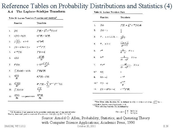
Reference Tables on Probability Distributions and Statistics (4) Source: Arnold O. Allen, Probability, Statistics, and Queueing Theory with Computer Science Applications, Academic Press, 1990 IR&DM, WS'11/12 October 20, 2011 II. 39