Chapter Five Risk Return and the Historical Record

Chapter Five Risk, Return, and the Historical Record INVESTMENTS | BODIE, KANE, MARCUS Copyright © 2014 Mc. Graw-Hill Education. All rights reserved. No reproduction or distribution without the prior written consent of Mc. Graw-Hill Education.

Chapter Overview • • • Interest rate determinants Rates of return for different holding periods Risk and risk premiums Estimations of return and risk Normal distribution • Deviation from normality and risk estimation • Historic returns on risky portfolios 5 -2 INVESTMENTS | BODIE, KANE, MARCUS

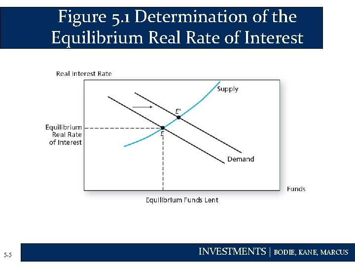
Interest Rate Determinants • Supply • Households • Demand • Businesses • Government’s net demand • Federal Reserve actions 5 -3 INVESTMENTS | BODIE, KANE, MARCUS

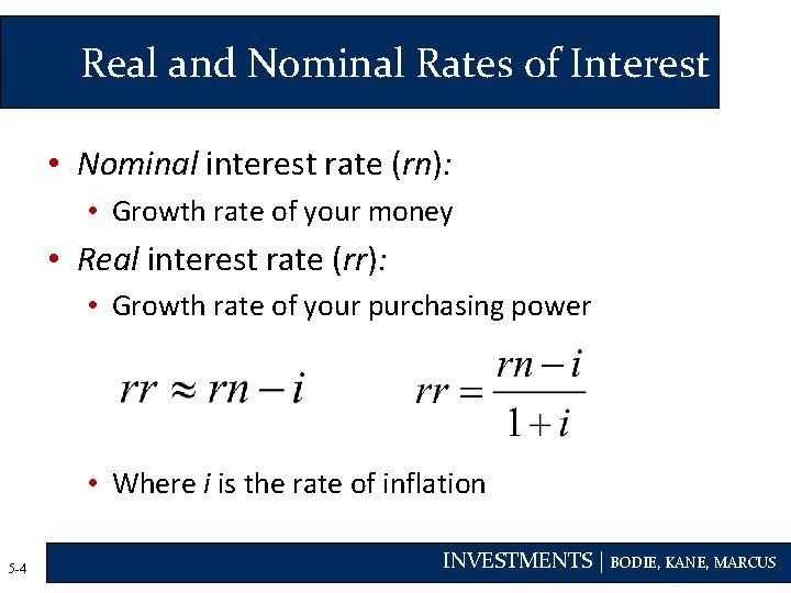
Real and Nominal Rates of Interest • Nominal interest rate (rn): • Growth rate of your money • Real interest rate (rr): • Growth rate of your purchasing power • Where i is the rate of inflation 5 -4 INVESTMENTS | BODIE, KANE, MARCUS

Figure 5. 1 Determination of the Equilibrium Real Rate of Interest 5 -5 INVESTMENTS | BODIE, KANE, MARCUS

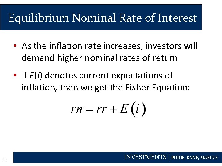
Equilibrium Nominal Rate of Interest • As the inflation rate increases, investors will demand higher nominal rates of return • If E(i) denotes current expectations of inflation, then we get the Fisher Equation: 5 -6 INVESTMENTS | BODIE, KANE, MARCUS

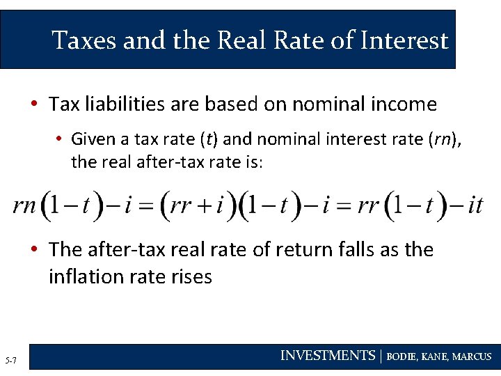
Taxes and the Real Rate of Interest • Tax liabilities are based on nominal income • Given a tax rate (t) and nominal interest rate (rn), the real after-tax rate is: • The after-tax real rate of return falls as the inflation rate rises 5 -7 INVESTMENTS | BODIE, KANE, MARCUS

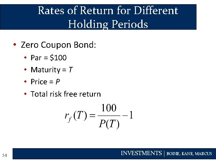
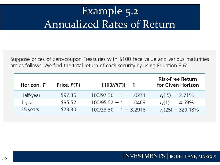
Rates of Return for Different Holding Periods • Zero Coupon Bond: • • 5 -8 Par = $100 Maturity = T Price = P Total risk free return INVESTMENTS | BODIE, KANE, MARCUS

Example 5. 2 Annualized Rates of Return 5 -9 INVESTMENTS | BODIE, KANE, MARCUS

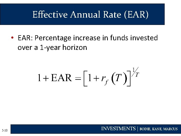
Effective Annual Rate (EAR) • EAR: Percentage increase in funds invested over a 1 -year horizon 5 -10 INVESTMENTS | BODIE, KANE, MARCUS

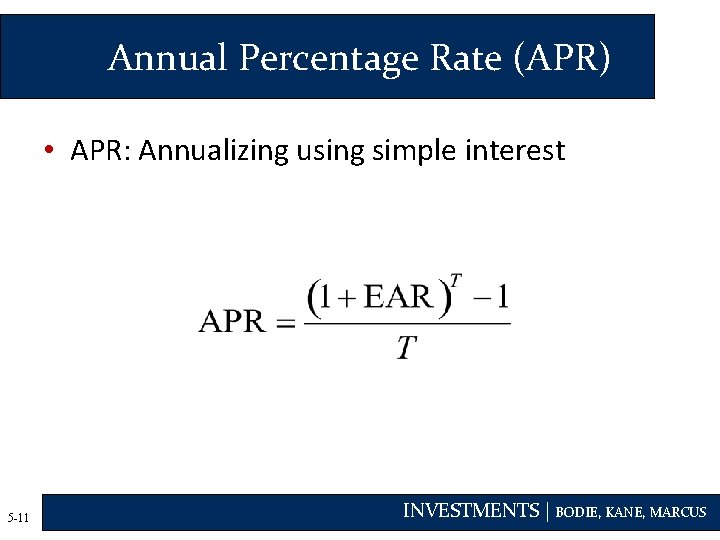
Annual Percentage Rate (APR) • APR: Annualizing using simple interest 5 -11 INVESTMENTS | BODIE, KANE, MARCUS

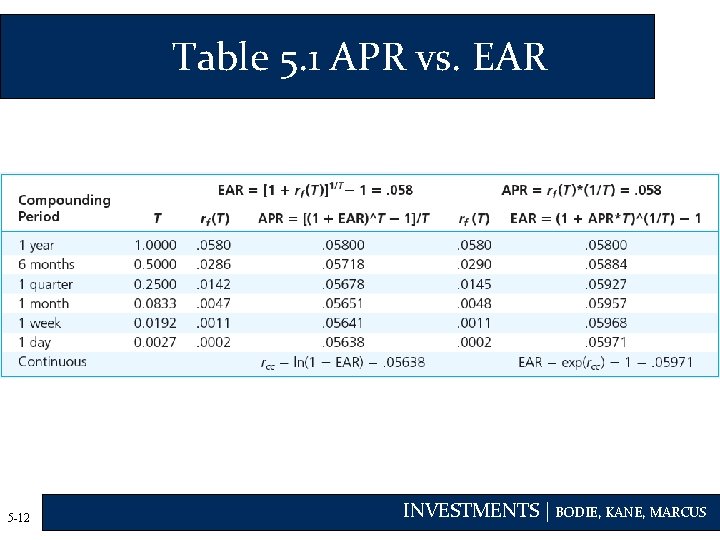
Table 5. 1 APR vs. EAR 5 -12 INVESTMENTS | BODIE, KANE, MARCUS

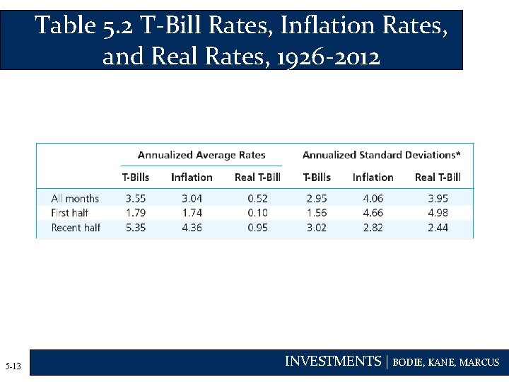
Table 5. 2 T-Bill Rates, Inflation Rates, and Real Rates, 1926 -2012 5 -13 INVESTMENTS | BODIE, KANE, MARCUS

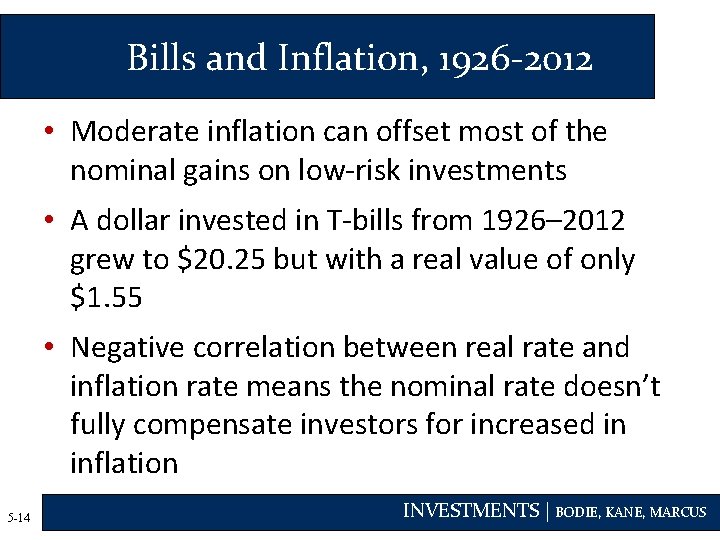
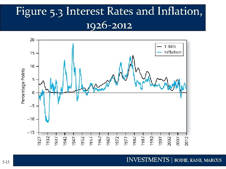
Bills and Inflation, 1926 -2012 • Moderate inflation can offset most of the nominal gains on low-risk investments • A dollar invested in T-bills from 1926– 2012 grew to $20. 25 but with a real value of only $1. 55 • Negative correlation between real rate and inflation rate means the nominal rate doesn’t fully compensate investors for increased in inflation 5 -14 INVESTMENTS | BODIE, KANE, MARCUS

Figure 5. 3 Interest Rates and Inflation, 1926 -2012 5 -15 INVESTMENTS | BODIE, KANE, MARCUS

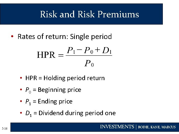
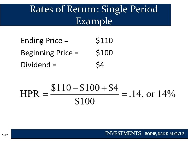
Risk and Risk Premiums • Rates of return: Single period • HPR = Holding period return • P 0 = Beginning price • P 1 = Ending price • D 1 = Dividend during period one 5 -16 INVESTMENTS | BODIE, KANE, MARCUS

Rates of Return: Single Period Example Ending Price = Beginning Price = Dividend = 5 -17 $110 $100 $4 INVESTMENTS | BODIE, KANE, MARCUS

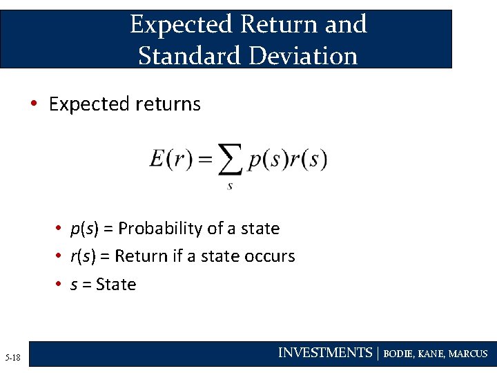
Expected Return and Standard Deviation • Expected returns • p(s) = Probability of a state • r(s) = Return if a state occurs • s = State 5 -18 INVESTMENTS | BODIE, KANE, MARCUS

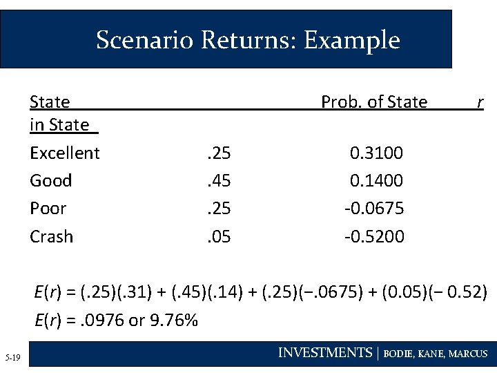
Scenario Returns: Example State in State Excellent Good Poor Crash Prob. of State. 25. 45. 25. 05 r 0. 3100 0. 1400 -0. 0675 -0. 5200 E(r) = (. 25)(. 31) + (. 45)(. 14) + (. 25)(−. 0675) + (0. 05)(− 0. 52) E(r) =. 0976 or 9. 76% 5 -19 INVESTMENTS | BODIE, KANE, MARCUS

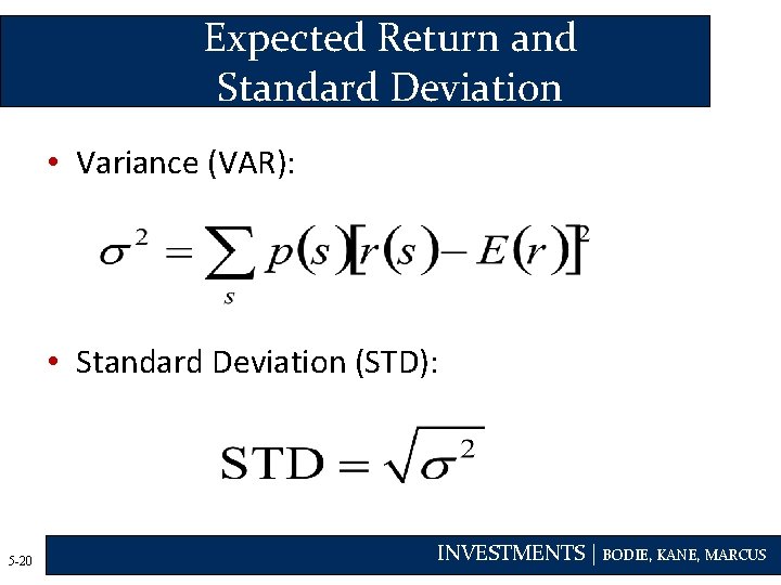
Expected Return and Standard Deviation • Variance (VAR): • Standard Deviation (STD): 5 -20 INVESTMENTS | BODIE, KANE, MARCUS

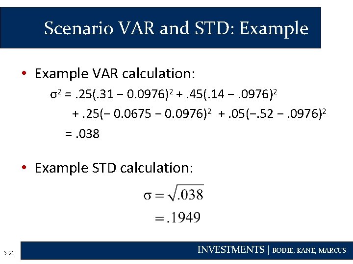
Scenario VAR and STD: Example • Example VAR calculation: σ2 =. 25(. 31 − 0. 0976)2 +. 45(. 14 −. 0976)2 +. 25(− 0. 0675 − 0. 0976)2 +. 05(−. 52 −. 0976)2 =. 038 • Example STD calculation: 5 -21 INVESTMENTS | BODIE, KANE, MARCUS

Time Series Analysis of Past Rates of Return • True means and variances are unobservable because we don’t actually know possible scenarios like the one in the examples • So we must estimate them (the means and variances, not the scenarios) 5 -22 INVESTMENTS | BODIE, KANE, MARCUS

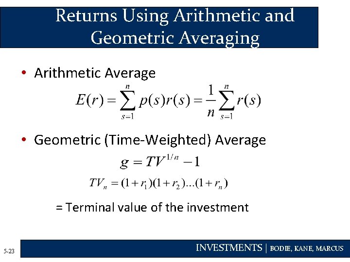
Returns Using Arithmetic and Geometric Averaging • Arithmetic Average • Geometric (Time-Weighted) Average = Terminal value of the investment 5 -23 INVESTMENTS | BODIE, KANE, MARCUS

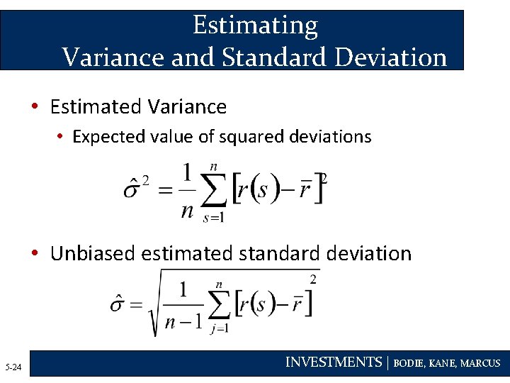
Estimating Variance and Standard Deviation • Estimated Variance • Expected value of squared deviations • Unbiased estimated standard deviation 5 -24 INVESTMENTS | BODIE, KANE, MARCUS

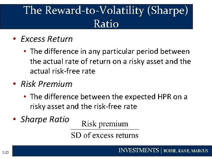
The Reward-to-Volatility (Sharpe) Ratio • Excess Return • The difference in any particular period between the actual rate of return on a risky asset and the actual risk-free rate • Risk Premium • The difference between the expected HPR on a risky asset and the risk-free rate • Sharpe Ratio 5 -25 INVESTMENTS | BODIE, KANE, MARCUS

The Normal Distribution • Investment management is easier when returns are normal • Standard deviation is a good measure of risk when returns are symmetric • If security returns are symmetric, portfolio returns will be as well • Future scenarios can be estimated using only the mean and the standard deviation • The dependence of returns across securities can be summarized using only the pairwise correlation coefficients 5 -26 INVESTMENTS | BODIE, KANE, MARCUS

Figure 5. 4 The Normal Distribution Mean = 10%, SD = 20% 5 -27 INVESTMENTS | BODIE, KANE, MARCUS

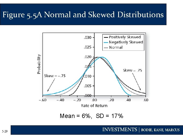
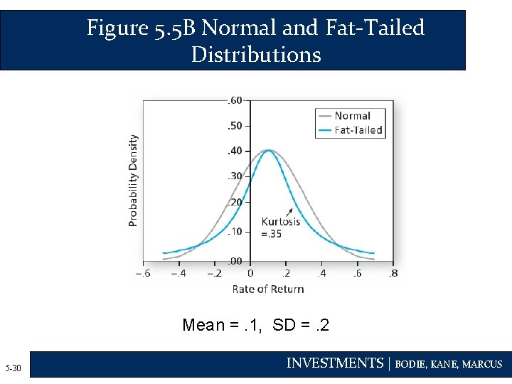
Normality and Risk Measures • What if excess returns are not normally distributed? • Standard deviation is no longer a complete measure of risk • Sharpe ratio is not a complete measure of portfolio performance • Need to consider skewness and kurtosis 5 -28 INVESTMENTS | BODIE, KANE, MARCUS

Figure 5. 5 A Normal and Skewed Distributions Mean = 6%, SD = 17% 5 -29 INVESTMENTS | BODIE, KANE, MARCUS

Figure 5. 5 B Normal and Fat-Tailed Distributions Mean =. 1, SD =. 2 5 -30 INVESTMENTS | BODIE, KANE, MARCUS

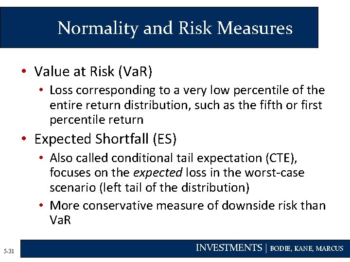
Normality and Risk Measures • Value at Risk (Va. R) • Loss corresponding to a very low percentile of the entire return distribution, such as the fifth or first percentile return • Expected Shortfall (ES) • Also called conditional tail expectation (CTE), focuses on the expected loss in the worst-case scenario (left tail of the distribution) • More conservative measure of downside risk than Va. R 5 -31 INVESTMENTS | BODIE, KANE, MARCUS

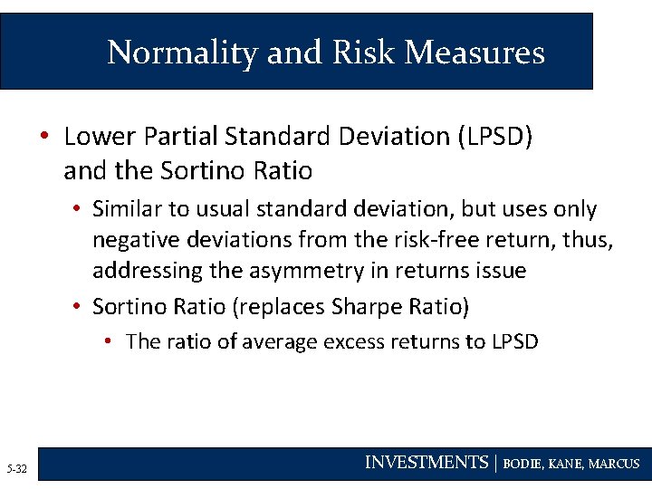
Normality and Risk Measures • Lower Partial Standard Deviation (LPSD) and the Sortino Ratio • Similar to usual standard deviation, but uses only negative deviations from the risk-free return, thus, addressing the asymmetry in returns issue • Sortino Ratio (replaces Sharpe Ratio) • The ratio of average excess returns to LPSD 5 -32 INVESTMENTS | BODIE, KANE, MARCUS

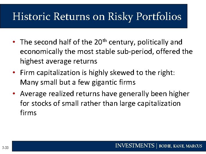
Historic Returns on Risky Portfolios • The second half of the 20 th century, politically and economically the most stable sub-period, offered the highest average returns • Firm capitalization is highly skewed to the right: Many small but a few gigantic firms • Average realized returns have generally been higher for stocks of small rather than large capitalization firms 5 -33 INVESTMENTS | BODIE, KANE, MARCUS

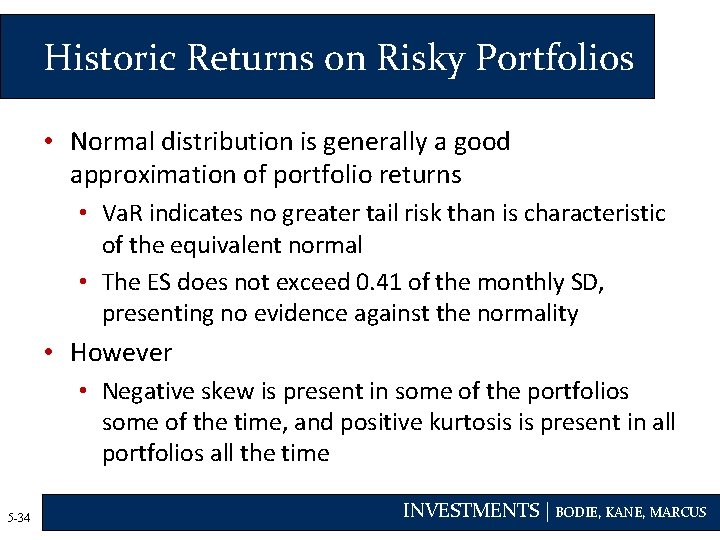
Historic Returns on Risky Portfolios • Normal distribution is generally a good approximation of portfolio returns • Va. R indicates no greater tail risk than is characteristic of the equivalent normal • The ES does not exceed 0. 41 of the monthly SD, presenting no evidence against the normality • However • Negative skew is present in some of the portfolios some of the time, and positive kurtosis is present in all portfolios all the time 5 -34 INVESTMENTS | BODIE, KANE, MARCUS

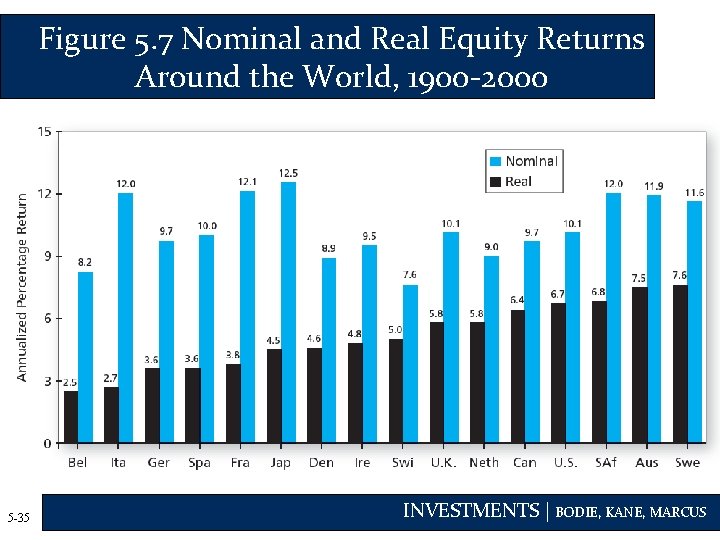
Figure 5. 7 Nominal and Real Equity Returns Around the World, 1900 -2000 5 -35 INVESTMENTS | BODIE, KANE, MARCUS

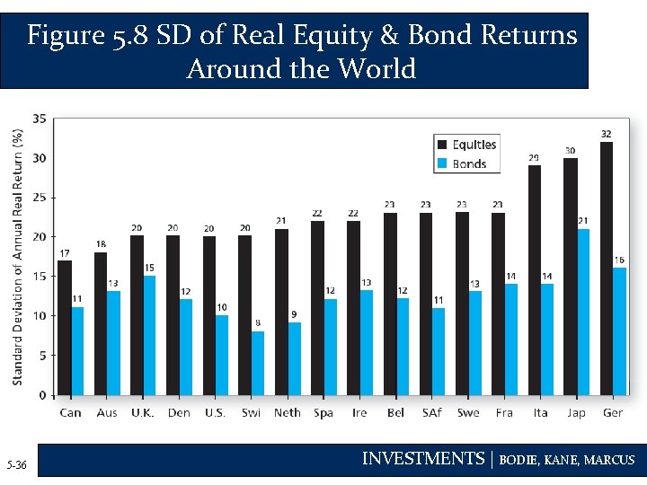
Figure 5. 8 SD of Real Equity & Bond Returns Around the World 5 -36 INVESTMENTS | BODIE, KANE, MARCUS

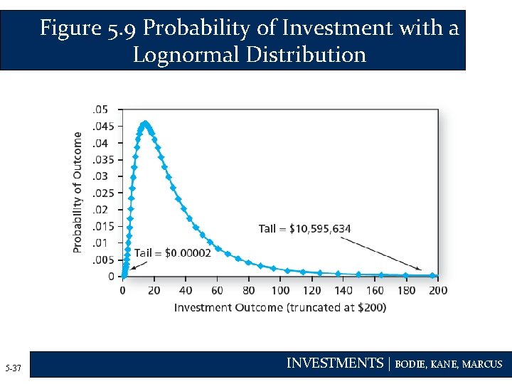
Figure 5. 9 Probability of Investment with a Lognormal Distribution 5 -37 INVESTMENTS | BODIE, KANE, MARCUS

Terminal Value with Continuous Compounding • When the continuously compounded rate of return on an asset is normally distributed, the effective rate of return will be lognormally distributed 5 -38 INVESTMENTS | BODIE, KANE, MARCUS