Chapter Five Applying Consumer Theory Topics Deriving Demand

Chapter Five Applying Consumer Theory

Topics § Deriving Demand Curves. § How Changes in Income Shift § Demand Curves. § Effects of a Price Change. § Cost-of-Living Adjustments. § Deriving Labor Supply Curves. © 2009 Pearson Addison-Wesley. All rights reserved. 2

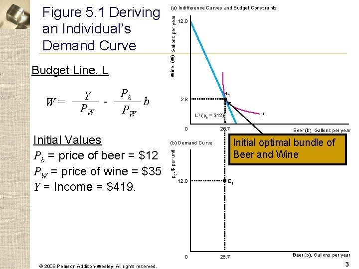
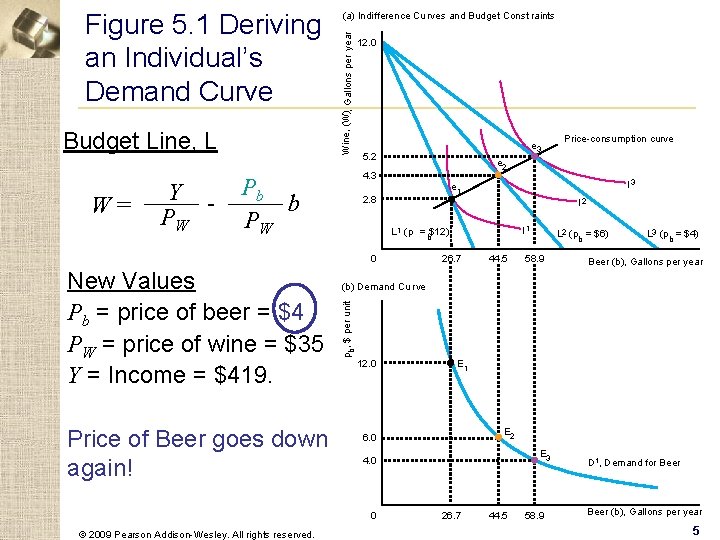
Budget Line, L W= Y PW Wine, (W), Gallons per year Figure 5. 1 Deriving an Individual’s Demand Curve (a) Indifference Cu rves and Budget Const raints Pb b PW 12. 0 e 1 2. 8 0 12. 0 0 © 2009 Pearson Addison-Wesley. All rights reserved. 26. 7 Beer (b), Gallons per year Initial optimal bundle of Beer and Wine (b) Demand Cu rve pb, $ per unit Initial Values Pb = price of beer = $12 PW = price of wine = $35 Y = Income = $419. I 1 L 1 (pb = $12) E 1 26. 7 Beer (b), Gallons per year 3

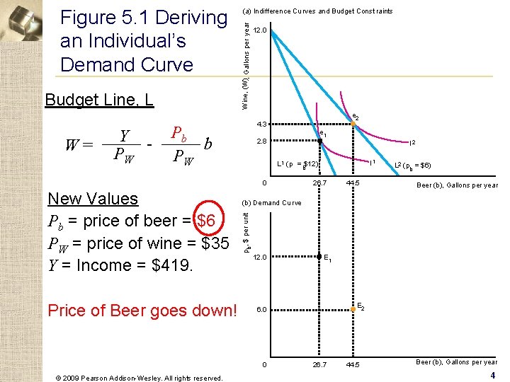
Budget Line, L W= Y PW Wine, (W), Gallons per year Figure 5. 1 Deriving an Individual’s Demand Curve (a) Indifference Cu rves and Budget Const raints 12. 0 e 2 4. 3 Pb b PW e 1 2. 8 I 2 0 Price of Beer goes down! 12. 0 44. 5 Beer (b), Gallons per year E 1 E 2 6. 0 0 © 2009 Pearson Addison-Wesley. All rights reserved. 26. 7 L 2 (pb = $6) (b) Demand Cu rve pb, $ per unit New Values Pb = price of beer = $6 PW = price of wine = $35 Y = Income = $419. I 1 L 1 (p = b$12) 26. 7 44. 5 Beer (b), Gallons per year 4

Budget Line, L W= Y PW Wine, (W), Gallons per year Figure 5. 1 Deriving an Individual’s Demand Curve (a) Indifference Cu rves and Budget Const raints 12. 0 e 3 5. 2 e 2 4. 3 Pb b PW Price of Beer goes down again! 2. 8 I 2 I 1 L 1 (p = b$12) 26. 7 44. 5 L 2 (pb = $6) 58. 9 L 3 (pb = $4) Beer (b), Gallons per year pb, $ per unit (b) Demand Cu rve 12. 0 E 1 E 2 6. 0 E 3 4. 0 0 © 2009 Pearson Addison-Wesley. All rights reserved. I 3 e 1 0 New Values Pb = price of beer = $4 PW = price of wine = $35 Y = Income = $419. Price-consumption curve 26. 7 44. 5 58. 9 D 1, Demand for Beer (b), Gallons per year 5

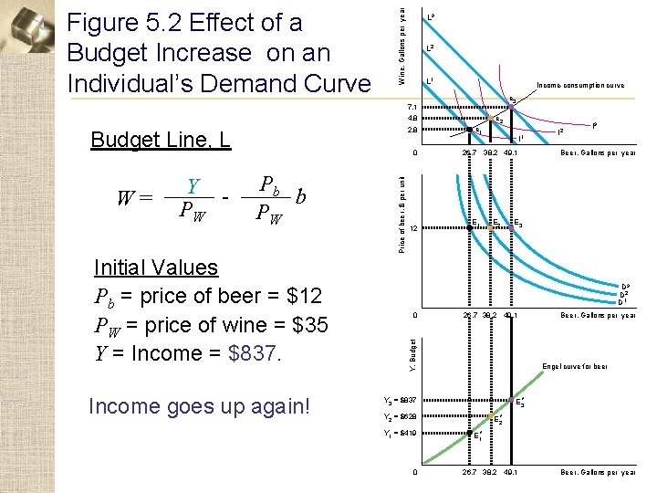
Effects of a Rise in Income § Engel curve - the relationship between the quantity demanded of a single good and income, holding prices constant © 2009 Pearson Addison-Wesley. All rights reserved. 6

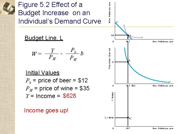
Win e, Gallons per year Figure 5. 2 Effect of a Budget Increase on an Individual’s Demand Curve 2. 8 Budget Line, L Pb b PW Initial Values Pb = price of beer = $12 PW = price of wine = $35 $628 Y = Income = $419. Price of bee r, $ per unit 0 12 e 1 26. 7 I 1 Beer, Gallons per year E 1 D 1 0 26. 7 38. 2 Beer, Gallons per year Y, Budget W= Y PW L 1 Income goes up! Y 1 = $419 0 E 1* 26. 7 Beer, Gallons per year

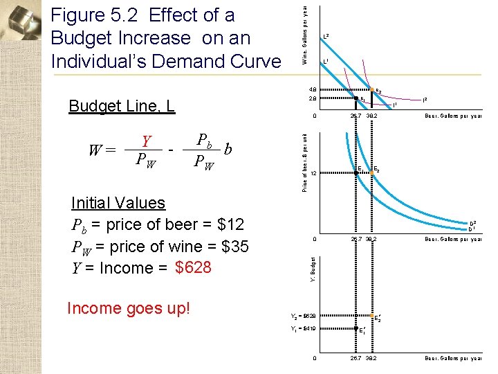
Win e, Gallons per year Figure 5. 2 Effect of a Budget Increase on an Individual’s Demand Curve L 2 L 1 e 2 4. 8 2. 8 Budget Line, L Initial Values Pb = price of beer = $12 PW = price of wine = $35 $628 Y = Income = $419. Income goes up! Price of bee r, $ per unit Pb b PW 12 I 1 26. 7 38. 2 E 1 I 2 Beer, Gallons per year E 2 D 1 0 26. 7 38. 2 Beer, Gallons per year Y, Budget W= Y PW 0 e 1 Y 2 = $628 Y 1 = $419 0 E 2* E 1* 26. 7 38. 2 Beer, Gallons per year

Win e, Gallons per year Figure 5. 2 Effect of a Budget Increase on an Individual’s Demand Curve L 3 L 2 L 1 Income-consumption curve e 3 7. 1 4. 8 2. 8 Budget Line, L Initial Values Pb = price of beer = $12 PW = price of wine = $35 Y = Income = $837. Income goes up again! Price of bee r, $ per unit Pb b PW 12 I 1 26. 7 38. 2 49. 1 E 2 I 3 Beer, Gallons per year E 3 D 2 D 1 0 26. 7 38. 2 49. 1 Y, Budget W= Y PW 0 e 2 e 1 Engel curve for beer E 3* Y 3 = $837 Y 2 = $628 Y 1 = $419 0 Beer, Gallons per year E 2* E 1* 26. 7 38. 2 49. 1 Beer, Gallons per year

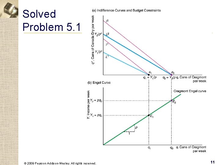
Solved Problem 5. 1 § Mahdu views Cragmont and Canada Dry ginger ales as perfect substitutes: He is indifferent as to which one he drinks. The price of a 12 -ounce can of Cragmont, p, is less than the price of a 12 -ounce can of Canada Dry, p*. What does Mahdu’s Engel curve for Cragmont ginger ale look like? How much does his weekly ginger ale budget have to rise for Mahdu to buy one more can of Cragmont ginger ale per week? © 2009 Pearson Addison-Wesley. All rights reserved. 10

Solved Problem 5. 1 © 2009 Pearson Addison-Wesley. All rights reserved. 11

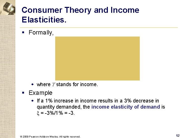
Consumer Theory and Income Elasticities. § Formally, w where Y stands for income. § Example w If a 1% increase in income results in a 3% decrease in quantity demanded, the income elasticity of demand is x = -3%/1% = -3. © 2009 Pearson Addison-Wesley. All rights reserved. 12

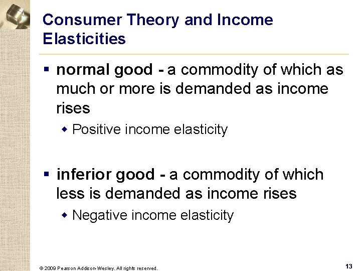
Consumer Theory and Income Elasticities § normal good - a commodity of which as much or more is demanded as income rises w Positive income elasticity § inferior good - a commodity of which less is demanded as income rises w Negative income elasticity © 2009 Pearson Addison-Wesley. All rights reserved. 13

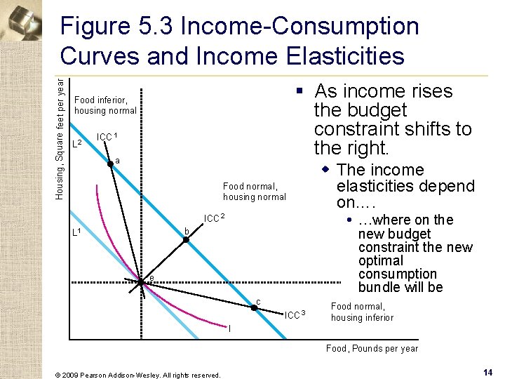
Housing, Square feet per year Figure 5. 3 Income-Consumption Curves and Income Elasticities § As income rises the budget constraint shifts to the right. Food inferior, housing normal L 2 ICC 1 a Food normal, housing normal ICC 2 …where on the new budget constraint the new optimal consumption bundle will be b L 1 w The income elasticities depend on…. e c ICC 3 Food normal, housing inferior I Food, Pounds per year © 2009 Pearson Addison-Wesley. All rights reserved. 14

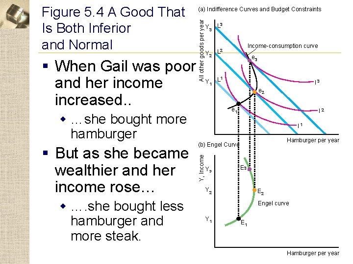
§ When Gail was poor and her income increased. . (a) Indifference Curves and Budget Constraints All other goods per year Figure 5. 4 A Good That Is Both Inferior and Normal Y 3 L 3 Y 2 w …. she bought less hamburger and more steak. e 3 1 Y 1 L I 3 e 2 e 1 w …she bought more hamburger I 2 I 1 Hamburger per year (b) Engel Curve Y, Income § But as she became wealthier and her income rose… Income-consumption curve L 2 Y 3 E 3 Y 2 Engel curve Y 1 E 1 Hamburger per year

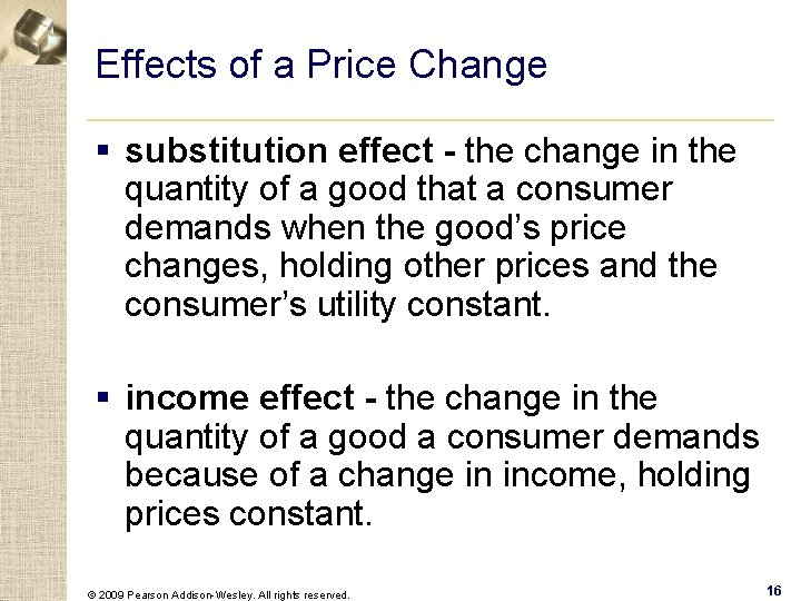
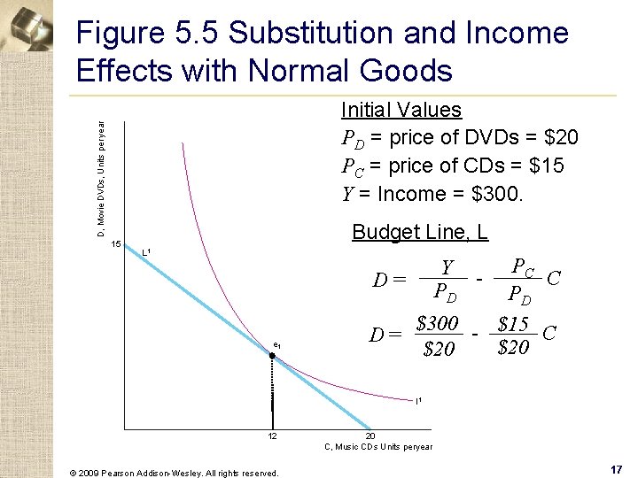
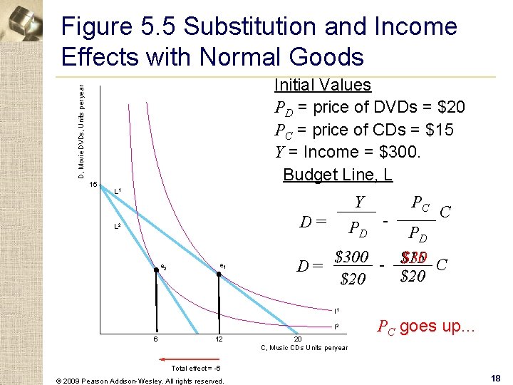
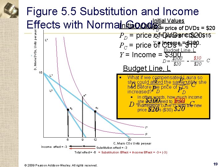
Effects of a Price Change § substitution effect - the change in the quantity of a good that a consumer demands when the good’s price changes, holding other prices and the consumer’s utility constant. § income effect - the change in the quantity of a good a consumer demands because of a change in income, holding prices constant. © 2009 Pearson Addison-Wesley. All rights reserved. 16

Figure 5. 5 Substitution and Income Effects with Normal Goods D, Movie DVDs, Units per year Initial Values PD = price of DVDs = $20 PC = price of CDs = $15 Y = Income = $300. 15 Budget Line, L L 1 PC C D= PD $300 - $15 C D= $20 Y PD e 1 I 1 12 © 2009 Pearson Addison-Wesley. All rights reserved. 20 C, Music CDs Units peryear 17

Figure 5. 5 Substitution and Income Effects with Normal Goods D, Movie DVDs, Units per year Initial Values PD = price of DVDs = $20 PC = price of CDs = $15 Y = Income = $300. Budget Line, L 15 L 1 Y PD - D= L 2 e 1 PC C PD $300 - $15 $30 C D= $20 I 1 I 2 6 12 20 C, Music CDs Units peryear PC goes up… Total effect = -6 © 2009 Pearson Addison-Wesley. All rights reserved. 18

Figure 5. 5 Substitution and Income Initial Values Effects with Normal. Initial Goods P = price of DVDs = $20 D, Movie DVDs, Units per year D price of = CDs = $15 PD = price Pof $20 C =DVDs Income = $300. PC = price Yof= CDs = $15 Budget Line, L Y = Income = $300 C D= $20 Budget Line, L L* 15 L 1 § L 2 e* e 1 e 2 What if we compensated Laura so PCutility she Y the she could afford same D before = Pthe price of CDs C had PD increased? D w In other words, how much income she would need to afford indifference curve I 1, with the new price of CDs ($30) $300 - $30 C D= $20 I 1 I 2 6 Income effect = -3 9 12 20 C, Music CDs Units peryear Substitution effect = -3 Total effect = -6 = Substitution Effect + Income Effect = -3 + (-3) © 2009 Pearson Addison-Wesley. All rights reserved. 19

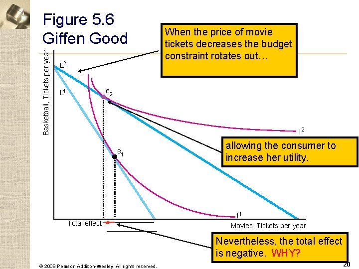
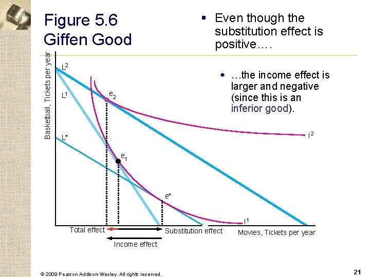
Basketball, Tickets per year Figure 5. 6 Giffen Good L 2 When the price of movie tickets decreases the budget constraint rotates out… e 2 L 1 I 2 e 1 Total effect allowing the consumer to increase her utility. I 1 Movies, Tickets per year Nevertheless, the total effect is negative. WHY? © 2009 Pearson Addison-Wesley. All rights reserved. 20

§ Even though the substitution effect is positive…. Basketball, Tickets per year Figure 5. 6 Giffen Good L 2 w …the income effect is larger and negative (since this is an inferior good). e 2 L 1 I 2 L* e 1 e* Total effect Substitution effect I 1 Movies, Tickets per year Income effect © 2009 Pearson Addison-Wesley. All rights reserved. 21

Inflation Indexes § Inflation - the increase in the overall price level over time. w nominal price - the actual price of a good. w real price - the price adjusted for inflation. § How do we adjust for inflation to calculate the real price? © 2009 Pearson Addison-Wesley. All rights reserved. 22

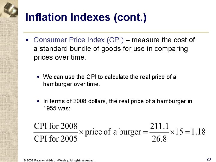
Inflation Indexes (cont. ) § Consumer Price Index (CPI) – measure the cost of a standard bundle of goods for use in comparing prices over time. w We can use the CPI to calculate the real price of a hamburger over time. w In terms of 2008 dollars, the real price of a hamburger in 1955 was: © 2009 Pearson Addison-Wesley. All rights reserved. 23

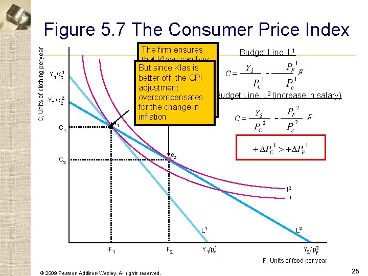
Effects of Inflation Adjustments § Scenario: Klaas signed a long-term contract when he was hired. According to the COLA clause in his contract, his employer increases his salary each year by the same percentage as that by which the CPI increases. If the CPI this year is 5% higher than the CPI last year, Klaas’s salary rises automatically by 5% over last year’s. § Question: what is the difference between using the CPI to adjust the long-term contract and using a true cost-of-living adjustment, which holds utility constant? © 2009 Pearson Addison-Wesley. All rights reserved. 24

C, Units of clothing per year Figure 5. 7 The Consumer Price Index Y 1 /p. C 1 Y 2 /p. C 2 C 1 e 1 The firm ensures Budget Line, L 1 that Klaas can buy Y 1 But is of thesince same. Klas bundle F C= better off, the CPI goods in adjustment second year that he Budget Line, L 2 (increase in salary) overcompensates chose in the first for the change in year… Y 2 inflation F C= - e 2 C 2 I 1 L 1 F 2 Y 1/p. F 1 L 2 Y 2 /p. F 2 F, Units of food per year © 2009 Pearson Addison-Wesley. All rights reserved. 25

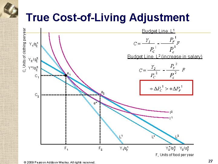
True Cost-of-Living Adjustment § True cost-of-living index - an inflation index that holds utility constant over time. § Question: how big an increase in Klaas’s salary would leave him exactly as well off in the second year as in the first? © 2009 Pearson Addison-Wesley. All rights reserved. 26

C, Units of clothing per year True Cost-of-Living Adjustment Budget Line, L 1 C= Y 1 /p. C 1 - F Budget Line, L 2 (increase in salary) Y 2 /p. C 2 Y* /p. C 2 Y 1 C= e 1 Y 2 - F e 2 C 2 e* I 2 I 1 L 1 F 2 Y 1/p. F 1 L* L 2 Y 2* /p. F 2 Y 2 /p. F 2 F, Units of food per year © 2009 Pearson Addison-Wesley. All rights reserved. 27

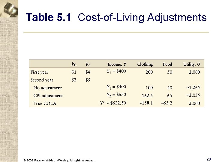
Table 5. 1 Cost-of-Living Adjustments © 2009 Pearson Addison-Wesley. All rights reserved. 28

Labor-Leisure Choice § Leisure - all time spent not working. § The number of hours worked per day, H, equals 24 minus the hours of leisure or nonwork, N, in a day: H = 24 − N. w The price of leisure is forgone earnings. The higher your wage, the more an hour of leisure costs you. © 2009 Pearson Addison-Wesley. All rights reserved. 29

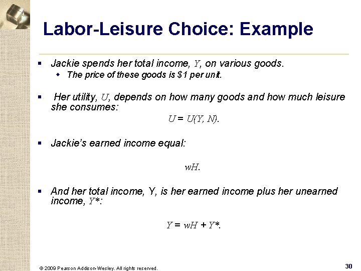
Labor-Leisure Choice: Example § Jackie spends her total income, Y, on various goods. w The price of these goods is $1 per unit. § Her utility, U, depends on how many goods and how much leisure she consumes: U = U(Y, N). § Jackie’s earned income equal: w. H. § And her total income, Y, is her earned income plus her unearned income, Y*: Y = w. H + Y*. © 2009 Pearson Addison-Wesley. All rights reserved. 30

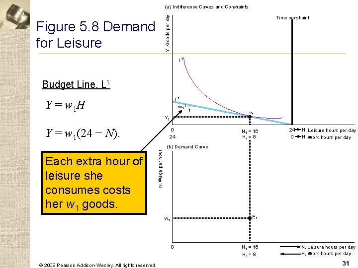
(a) Indifference Curves and Constraints Y, Goods per day Time constraint Figure 5. 8 Demand for Leisure I 1 Budget Line, L 1 –w 1 Y = w 1 H 1 Y = w 1(24 − N). 0 24 e 1 N 1 = 16 H 1 = 8 24 0 N, Leisure hours per day H, Work hours per day Each extra hour of leisure she consumes costs her w 1 goods. w, Wage per hour (b) Demand Curve E 1 w 1 0 © 2009 Pearson Addison-Wesley. All rights reserved. N 1 = 16 H 1 = 8 N, Leisure hours per day H, Work hours per day 31

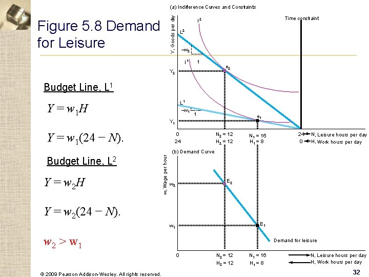
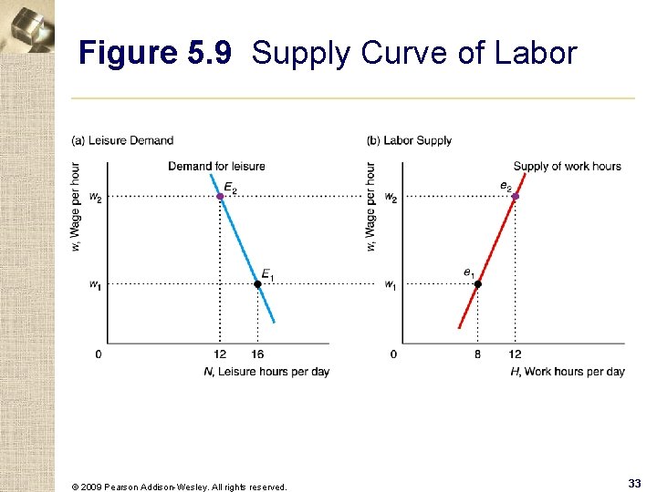
Y, Goods per day (a) Indifference Curves and Constraints Figure 5. 8 Demand for Leisure Time constraint I 2 L 2 –w 2 1 I 1 Y 2 e 2 Budget Line, L 1 –w 1 Y = w 1 H 1 e 1 Y = w 1(24 − N). 0 24 N 2 = 12 H 2 = 12 N 1 = 16 H 1 = 8 24 0 N, Leisure hours per day H, Work hours per day Budget Line, L 2 Y = w 2 H w, Wage per hour (b) Demand Curve E 2 w 2 Y = w 2(24 − N). E 1 w 2 > w 1 Demand for leisure 0 © 2009 Pearson Addison-Wesley. All rights reserved. N 2 = 12 H 2 = 12 N 1 = 16 H 1 = 8 N, Leisure hours per day H, Work hours per day 32

Figure 5. 9 Supply Curve of Labor © 2009 Pearson Addison-Wesley. All rights reserved. 33

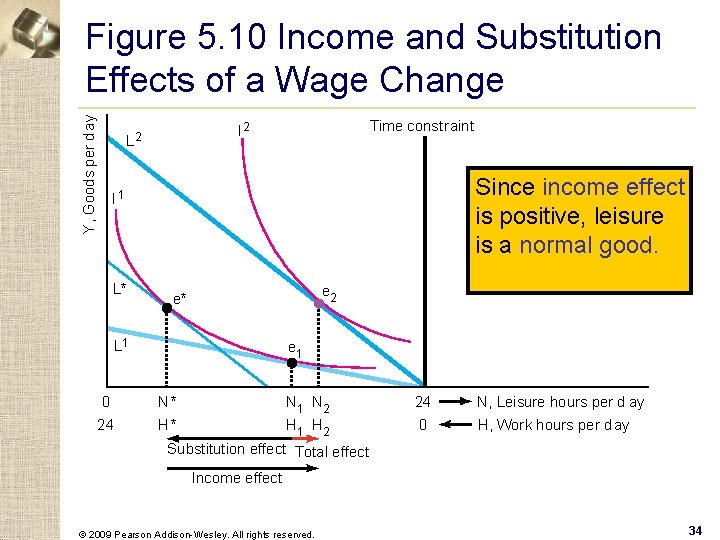
Y, Goods per d ay Figure 5. 10 Income and Substitution Effects of a Wage Change Time constraint I 2 L 2 Since income effect is positive, leisure is a normal good. I 1 L* e 2 e* L 1 e 1 0 N* N 1 N 2 24 N, Leisure hours per d ay 24 H* H 1 H 2 0 H, Work hours per d ay Substitution effect Total effect Income effect © 2009 Pearson Addison-Wesley. All rights reserved. 34

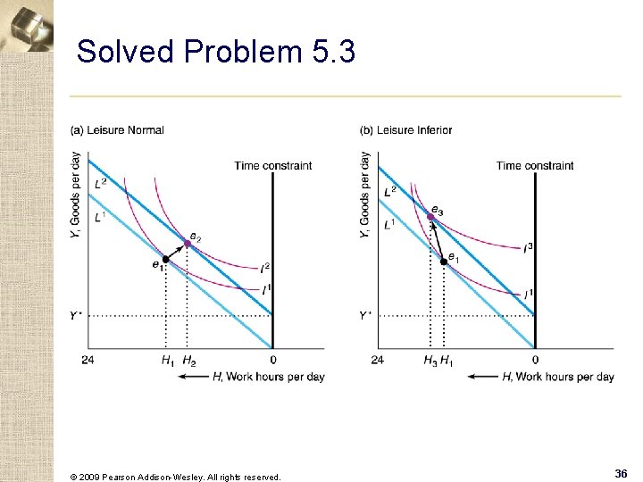
Solved Problem 5. 3 § Enrico receives a no-strings-attached scholarship that pays him an extra Y* per day. How does this scholarship affect the number of hours he wants to work? Does his utility increase? © 2009 Pearson Addison-Wesley. All rights reserved. 35

Solved Problem 5. 3 © 2009 Pearson Addison-Wesley. All rights reserved. 36

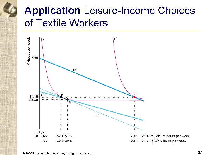
Application Leisure-Income Choices of Textile Workers © 2009 Pearson Addison-Wesley. All rights reserved. 37

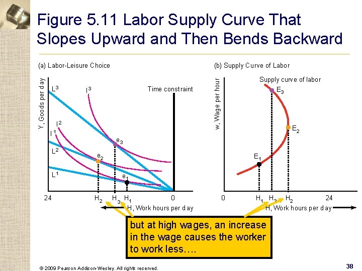
Figure 5. 11 Labor Supply Curve That Slopes Upward and Then Bends Backward L 3 (b) Supply Curve of Labor Time const raint I 3 I 2 I 1 L 2 E 3 E 2 e 3 e 2 E 1 L 1 24 Supply curve of labor w, Wage per hour Y, Goods per d ay (a) Labor-Leisure Choice e 1 H 2 H 3 H 1 0 H, Work hours per d ay 0 H 1 H 3 H 2 24 H, Work hours per d ay butlow At at high wages, an increase in the wage causes the worker to work to less…. work more…. © 2009 Pearson Addison-Wesley. All rights reserved. 38

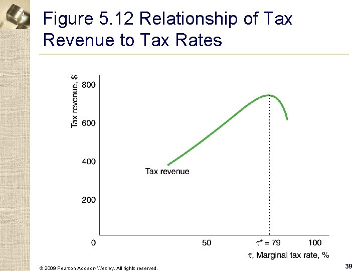
Figure 5. 12 Relationship of Tax Revenue to Tax Rates © 2009 Pearson Addison-Wesley. All rights reserved. 39

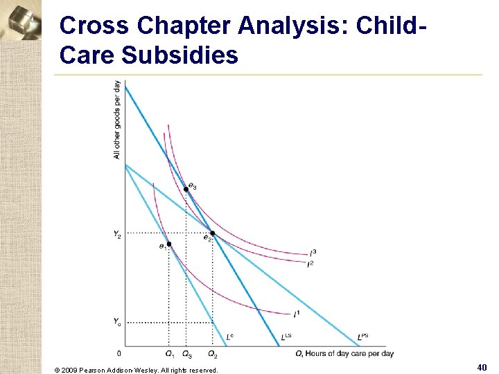
Cross Chapter Analysis: Child. Care Subsidies © 2009 Pearson Addison-Wesley. All rights reserved. 40