CHAPTER Fiscal Policy 30 After studying this chapter

CHAPTER Fiscal Policy 30

After studying this chapter you will be able to – Describe the federal budget process and the recent history of outlays, tax revenues, deficits, and debts – Explain the The Supply-Side: Employment and Potential GDP on employment and potential GDP – Explain the effects of deficits on investment, saving, and economic growth – Explain how fiscal policy choices redistribute benefits and costs across generations – Explain how fiscal policy can be used to stabilize the business cycle

Balancing Acts on Capitol Hill In 2007, the federal government planned to spend 21. 1 cents out of each dollar earned in the United States and collected 18. 2 cents per dollar in taxes. How does the government’s planned deficit affect the economy? Federal government deficits are not new. Apart from four years 1998 2001, the federal government has had a budget deficit. How do government deficits and the debt they bring affect the economy?

The Federal Budget The federal budget is the annual statement of the federal government’s outlays and tax revenues. The federal budget has two purposes: 1. To finance the activities of the federal government 2. To achieve macroeconomic objectives Fiscal policy is the use of the federal budget to achieve macroeconomic objectives, such as full employment, sustained economic growth, and price level stability.

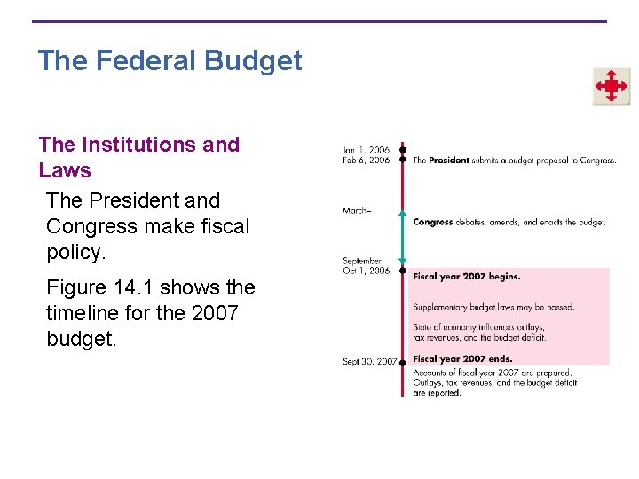
The Federal Budget The Institutions and Laws The President and Congress make fiscal policy. Figure 14. 1 shows the timeline for the 2007 budget.

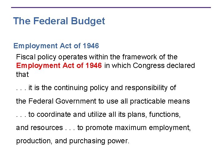
The Federal Budget Employment Act of 1946 Fiscal policy operates within the framework of the Employment Act of 1946 in which Congress declared that. . . it is the continuing policy and responsibility of the Federal Government to use all practicable means. . . to coordinate and utilize all its plans, functions, and resources. . . to promote maximum employment, production, and purchasing power.

The Federal Budget The Council of Economic Advisers monitors the economy and keeps the President and the public well informed about the current state of the economy and the best available forecasts of where it is heading. This economic intelligence activity is one source of data that informs the budget-making process.

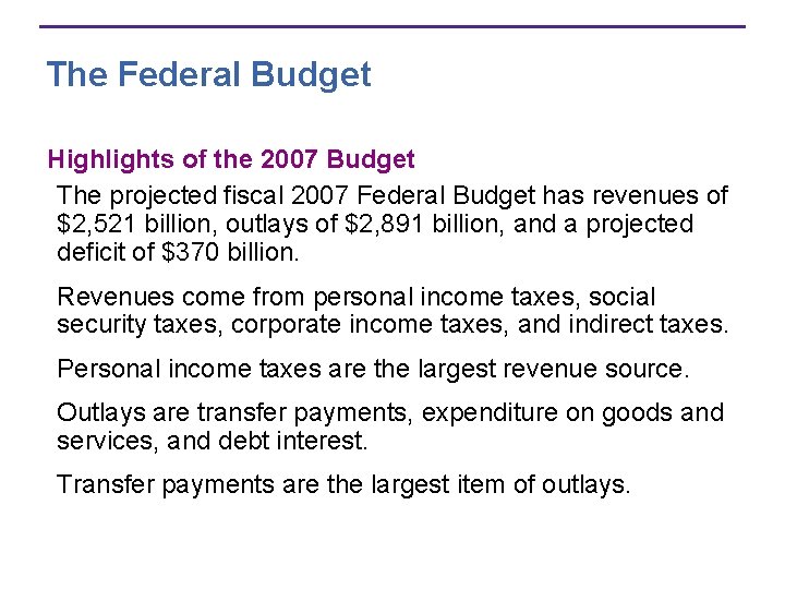
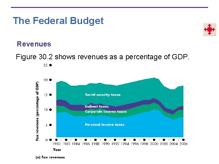
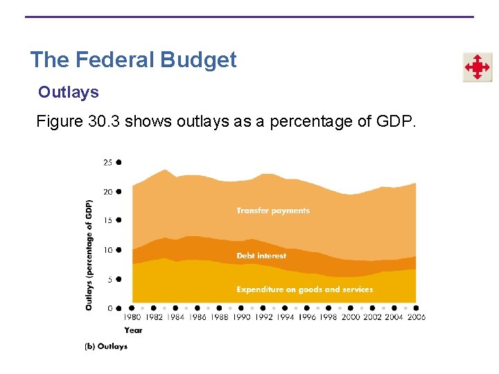
The Federal Budget Highlights of the 2007 Budget The projected fiscal 2007 Federal Budget has revenues of $2, 521 billion, outlays of $2, 891 billion, and a projected deficit of $370 billion. Revenues come from personal income taxes, social security taxes, corporate income taxes, and indirect taxes. Personal income taxes are the largest revenue source. Outlays are transfer payments, expenditure on goods and services, and debt interest. Transfer payments are the largest item of outlays.

The Federal Budget Surplus or Deficit The federal government’s budget balance equals tax revenue minus outlays. If revenues exceed outlays, the government has a budget surplus. If outlays exceed revenues, the government has a budget deficit. If revenues equal outlays, the government has a balanced budget. The projected budget deficit in fiscal 2007 is $370 billion.

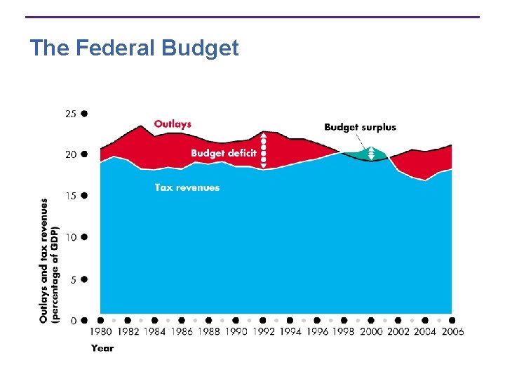
The Federal Budget The Budget in Historical Perspective Figure 30. 1 on the next slide shows the government’s tax revenues, outlays, and budget surplus or deficit as a percentage of GDP for the period 1980 to 2006. The government deficit peaked at 5. 2 percent of GDP in 1983. The deficit declined through 1989 but climbed again during the 1990– 1991 recession and then began to shrink. In 1998, a surplus emerged. But by 2002, the budget was again in deficit.

The Federal Budget

The Federal Budget Revenues Figure 30. 2 shows revenues as a percentage of GDP.

The Federal Budget Outlays Figure 30. 3 shows outlays as a percentage of GDP.

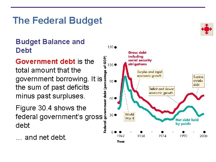
The Federal Budget Balance and Debt Government debt is the total amount that the government borrowing. It is the sum of past deficits minus past surpluses. Figure 30. 4 shows the federal government’s gross debt … and net debt.

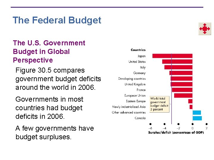
The Federal Budget The U. S. Government Budget in Global Perspective Figure 30. 5 compares government budget deficits around the world in 2006. Governments in most countries had budget deficits in 2006. A few governments have budget surpluses.

The Federal Budget State and Local Budgets The total government sector includes state and local governments as well as the federal government. In 2005, when federal government outlays were about $2, 500 billion, state and local outlays were almost $1, 700 billion. Most of state expenditures were on public schools, colleges, and universities ($550 billion); local police and fire services; and roads.

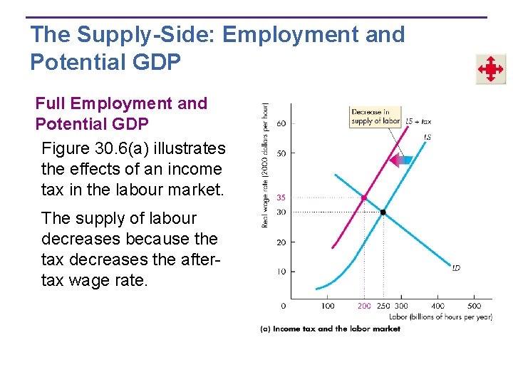
The Supply-Side: Employment and Potential GDP Fiscal policy has important effects employment, potential GDP, and aggregate supply—called supply-side effects. An income tax changes full employment and potential GDP.

The Supply-Side: Employment and Potential GDP Full Employment and Potential GDP Figure 30. 6(a) illustrates the effects of an income tax in the labour market. The supply of labour decreases because the tax decreases the aftertax wage rate.

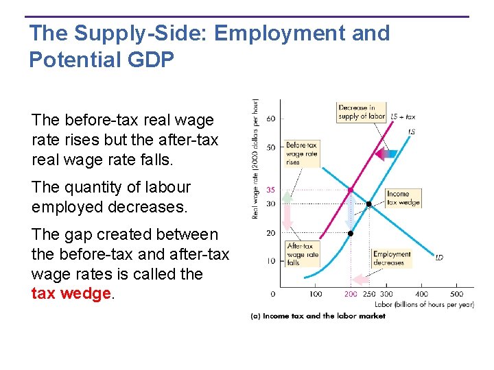
The Supply-Side: Employment and Potential GDP The before-tax real wage rate rises but the after-tax real wage rate falls. The quantity of labour employed decreases. The gap created between the before-tax and after-tax wage rates is called the tax wedge.

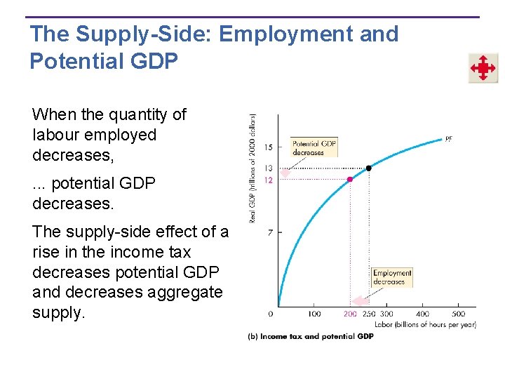
The Supply-Side: Employment and Potential GDP When the quantity of labour employed decreases, . . . potential GDP decreases. The supply-side effect of a rise in the income tax decreases potential GDP and decreases aggregate supply.

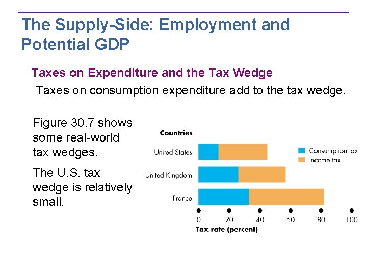
The Supply-Side: Employment and Potential GDP Taxes on Expenditure and the Tax Wedge Taxes on consumption expenditure add to the tax wedge. Figure 30. 7 shows some real-world tax wedges. The U. S. tax wedge is relatively small.

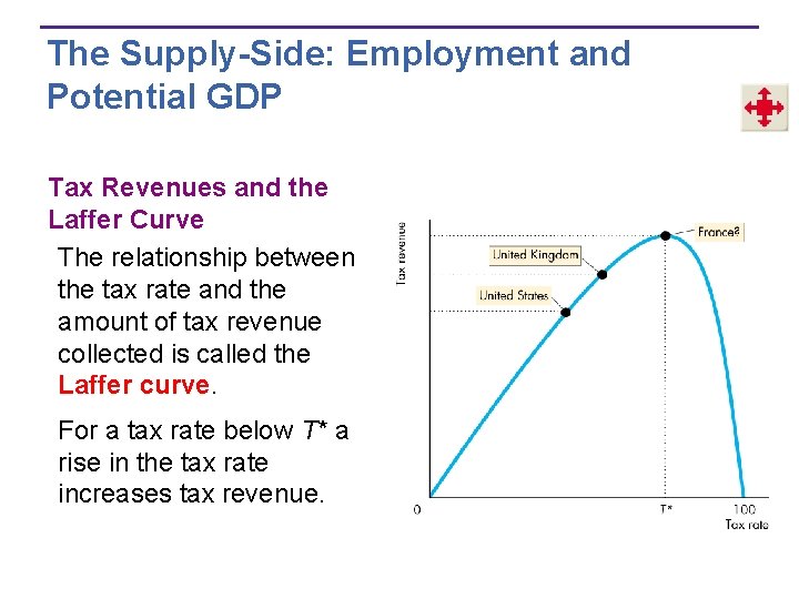
The Supply-Side: Employment and Potential GDP Tax Revenues and the Laffer Curve The relationship between the tax rate and the amount of tax revenue collected is called the Laffer curve. For a tax rate below T* a rise in the tax rate increases tax revenue.

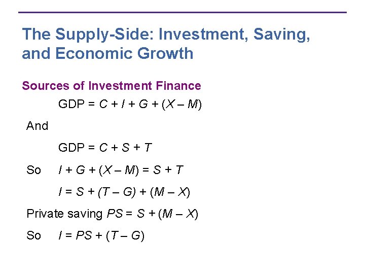
The Supply-Side: Investment, Saving, and Economic Growth Sources of Investment Finance GDP = C + I + G + (X – M) And GDP = C + S + T So I + G + (X – M) = S + T I = S + (T – G) + (M – X) Private saving PS = S + (M – X) So I = PS + (T – G)

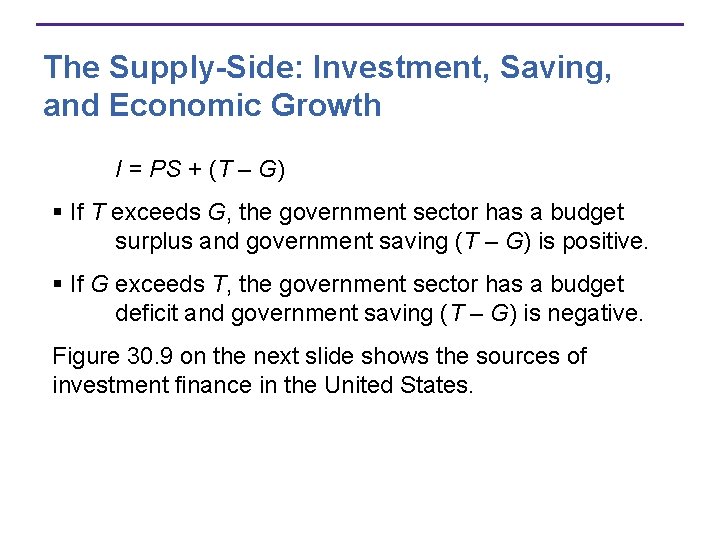
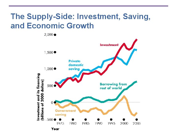
The Supply-Side: Investment, Saving, and Economic Growth I = PS + (T – G) § If T exceeds G, the government sector has a budget surplus and government saving (T – G) is positive. § If G exceeds T, the government sector has a budget deficit and government saving (T – G) is negative. Figure 30. 9 on the next slide shows the sources of investment finance in the United States.

The Supply-Side: Investment, Saving, and Economic Growth

The Supply-Side: Investment, Saving, and Economic Growth Fiscal policy influences investment and saving in two ways: § Taxes affect the incentive to save and change the supply of loanable funds. § Government saving is a component of total saving and the supply of loanable funds.

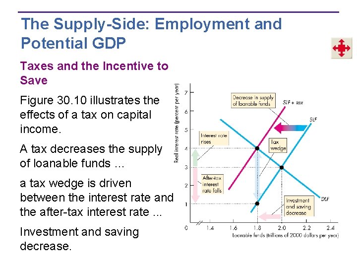
The Supply-Side: Employment and Potential GDP Taxes and the Incentive to Save Figure 30. 10 illustrates the effects of a tax on capital income. A tax decreases the supply of loanable funds … a tax wedge is driven between the interest rate and the after-tax interest rate. . . Investment and saving decrease.

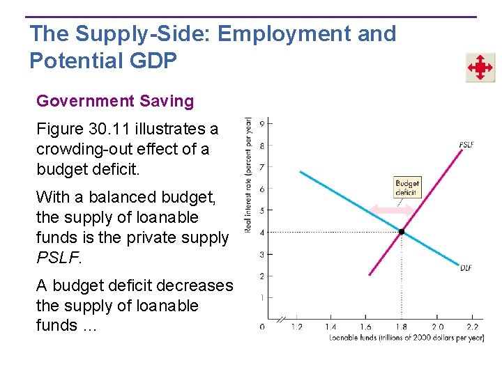
The Supply-Side: Employment and Potential GDP Government Saving Figure 30. 11 illustrates a crowding-out effect of a budget deficit. With a balanced budget, the supply of loanable funds is the private supply PSLF. A budget deficit decreases the supply of loanable funds …

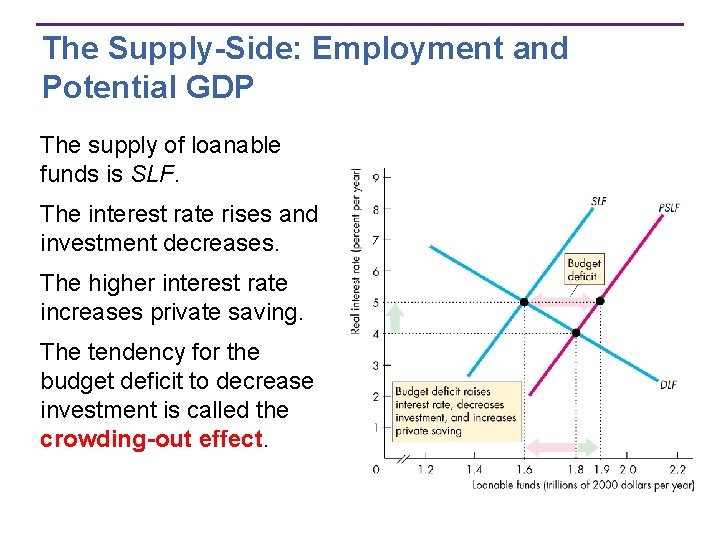
The Supply-Side: Employment and Potential GDP The supply of loanable funds is SLF. The interest rate rises and investment decreases. The higher interest rate increases private saving. The tendency for the budget deficit to decrease investment is called the crowding-out effect.

The Supply-Side: Employment and Potential GDP In the crowding-out case, the quantity of private saving changes along the PSLF curve as the real interest rate rises. But suppose that the budget deficit (government borrowing) changes private saving and shifts the PSLF curve. This possibility is called the Ricardo-Barro effect. Ricardo-Barro equivalence is the proposition that taxes and government borrowing are equivalent—budget deficit has no effect on the real interest rate or investment.

Generational Effects of Fiscal Policy Is the budget deficit a burden of future generations? Is the budget deficit the only burden of future generations? What about the deficit in the Social Security fund? Does it matter who owns the bonds that the government sells to finance its deficit? To answer questions like these, we use a tool called generation accounting. Generational accounting is an accounting system that measures the lifetime tax burden and benefits of each generation.

Generational Effects of Fiscal Policy Generational Accounting and Present Value Taxes are paid by people with jobs. Social security benefits are paid to people after they retire. So to compare the value of an amount of money at one date (working years) with that at a later date (retirement years), we use the concept of present value. A present value is an amount of money that, if invested today, will grow to equal a given future amount when the interest that it earns is taken into account. If the interest rate is 5 percent a year, $1, 000 invested in 2006 will grow, with interest, to $11, 467 after 50 years. The present value (in 2006) of $11, 467 in 2056 is $1, 000.

Generational Effects of Fiscal Policy The Social Security Time Bomb Using generational accounting and present values, economists have found that the federal government is facing a Social Security time bomb! In 2008, the first of the baby boomers will start collecting Social Security pensions and in 2011, they will become eligible for Medicare benefits. By 2030, all the baby boomers will have retired and, compared to 2006, the population supported by Social Security will have doubled.

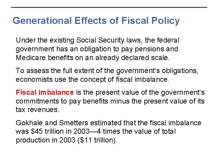
Generational Effects of Fiscal Policy Under the existing Social Security laws, the federal government has an obligation to pay pensions and Medicare benefits on an already declared scale. To assess the full extent of the government’s obligations, economists use the concept of fiscal imbalance. Fiscal imbalance is the present value of the government’s commitments to pay benefits minus the present value of its tax revenues. Gokhale and Smetters estimated that the fiscal imbalance was $45 trillion in 2003— 4 times the value of total production in 2003 ($11 trillion).

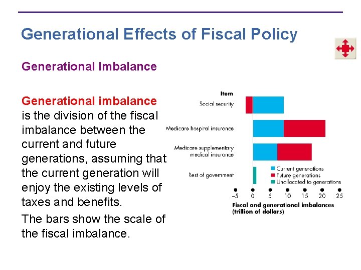
Generational Effects of Fiscal Policy Generational Imbalance Generational imbalance is the division of the fiscal imbalance between the current and future generations, assuming that the current generation will enjoy the existing levels of taxes and benefits. The bars show the scale of the fiscal imbalance.

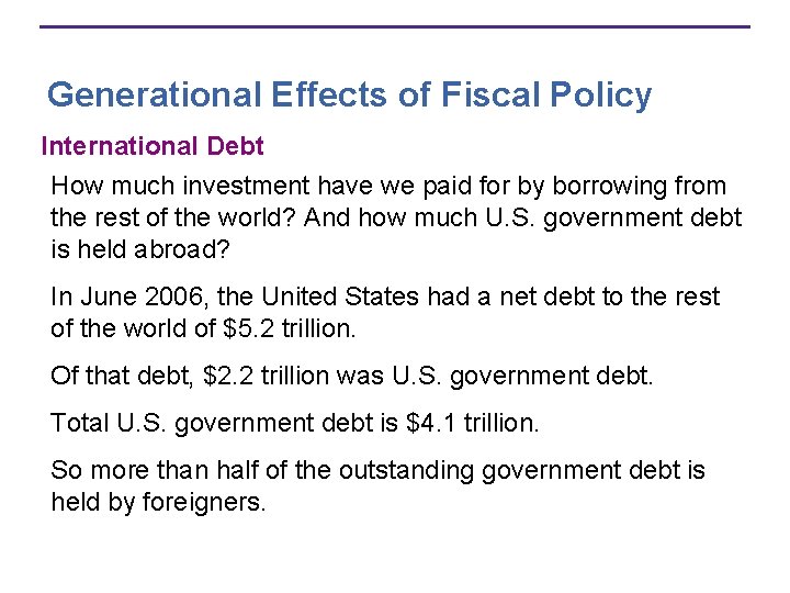
Generational Effects of Fiscal Policy International Debt How much investment have we paid for by borrowing from the rest of the world? And how much U. S. government debt is held abroad? In June 2006, the United States had a net debt to the rest of the world of $5. 2 trillion. Of that debt, $2. 2 trillion was U. S. government debt. Total U. S. government debt is $4. 1 trillion. So more than half of the outstanding government debt is held by foreigners.

Stabilizing the Business Cycle Fiscal policy actions that seek to stabilize the business cycle work by changing aggregate demand. ■ Discretionary or ■ Automatic Discretionary fiscal policy is a policy action that is initiated by an act of Congress. Automatic fiscal policy is a change in fiscal policy triggered by the state of the economy.

Stabilizing the Business Cycle The Government Expenditure Multiplier The government expenditure multiplier is the magnification effect of a change in government expenditure on goods and services on aggregate demand. A multiplier exists because government expenditure is a component of aggregate expenditure. An increase in government expenditure increases income, which induces additional consumption expenditure and which in turn increases aggregate demand.

Stabilizing the Business Cycle The Autonomous Tax Multiplier The autonomous tax multiplier is the magnification effect a change in autonomous taxes on aggregate demand. A decrease in autonomous taxes increases disposable income, which increases consumption expenditure and increases aggregate demand. The magnitude of the autonomous tax multiplier is smaller than the government expenditure multiplier because the a $1 tax cut induces less than a $1 increase in consumption expenditure.

Stabilizing the Business Cycle The Balanced Budget Multiplier The balanced tax multiplier is the magnification effect on aggregate demand of a simultaneous change in government expenditure and taxes that leaves the budget balance unchanged. The balanced budget multiplier is positive because a $1 increase in government expenditure increases aggregate demand by more than a $1 increase in taxes decreases aggregate demand. So when both government expenditure and taxes increase by $1, aggregate demand increases.

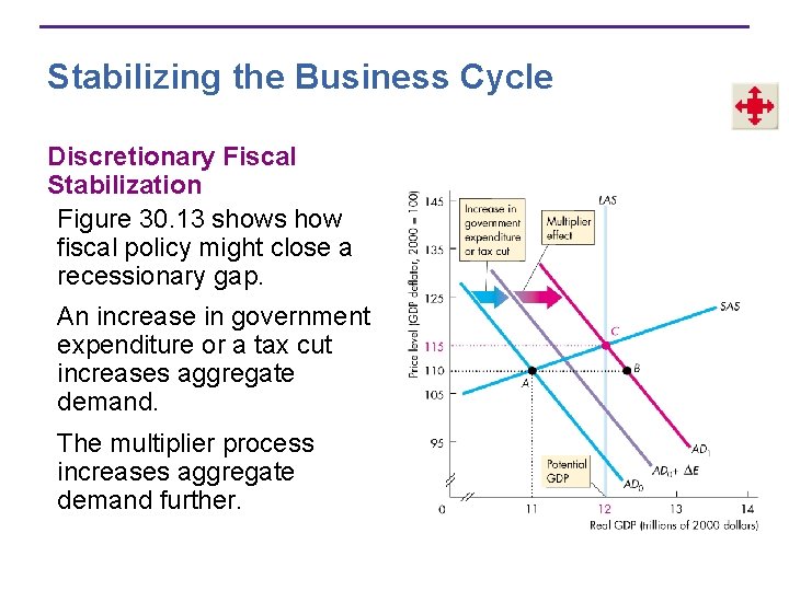
Stabilizing the Business Cycle Discretionary Fiscal Stabilization Figure 30. 13 shows how fiscal policy might close a recessionary gap. An increase in government expenditure or a tax cut increases aggregate demand. The multiplier process increases aggregate demand further.

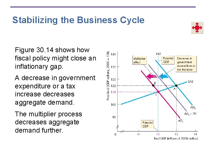
Stabilizing the Business Cycle Figure 30. 14 shows how fiscal policy might close an inflationary gap. A decrease in government expenditure or a tax increase decreases aggregate demand. The multiplier process decreases aggregate demand further.

Stabilizing the Business Cycle Limitations of Discretionary Fiscal Policy The use of discretionary fiscal policy is seriously hampered by three time lags: § Recognition lag—the time it takes to figure out that fiscal policy action is needed. § Law-making lag—the time it takes Congress to pass the laws needed to change taxes or spending. § Impact lag—the time it takes from passing a tax or spending change to its effect on real GDP being felt.

Stabilizing the Business Cycle Automatic Stabilizers Automatic stabilizers are mechanisms that stabilize real GDP without explicit action by the government. Induced taxes and needs-tested spending are automatic stabilizers. Taxes that vary with real GDP are called induced taxes. When real GDP increases in an expansion, wages and profits rise, so the taxes on these incomes—induced taxes —rise. When real GDP decreases in a recession, wages and profits fall, so the induced taxes on these incomes fall.

Stabilizing the Business Cycle The spending on programs that pay benefits to suitably qualified people and businesses is called needs-tested spending. When the economy is in a recession, unemployment is high and needs-tested spending on unemployment benefits and food stamps increases. When the economy expands, unemployment falls, and needs-tested spending decreases. Induced taxes and needs-tested spending decrease the multiplier effects of changes in autonomous expenditure. So they moderate both expansions and recessions and make real GDP more stable.

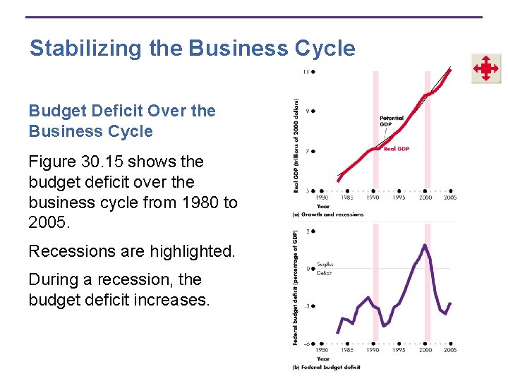
Stabilizing the Business Cycle Budget Deficit Over the Business Cycle Figure 30. 15 shows the budget deficit over the business cycle from 1980 to 2005. Recessions are highlighted. During a recession, the budget deficit increases.

Stabilizing the Business Cycle Cyclical and Structural Balances The structural surplus or deficit is the surplus or deficit that would occur if the economy were at full employment and real GDP were equal to potential GDP. The cyclical surplus or deficit is the actual surplus or deficit minus the structural surplus or deficit; that is, it is the surplus or deficit that occurs purely because real GDP does not equal potential GDP.

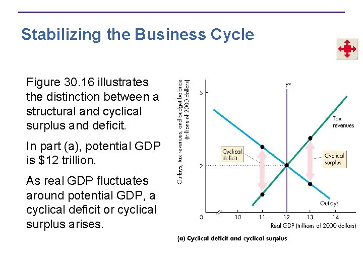
Stabilizing the Business Cycle Figure 30. 16 illustrates the distinction between a structural and cyclical surplus and deficit. In part (a), potential GDP is $12 trillion. As real GDP fluctuates around potential GDP, a cyclical deficit or cyclical surplus arises.

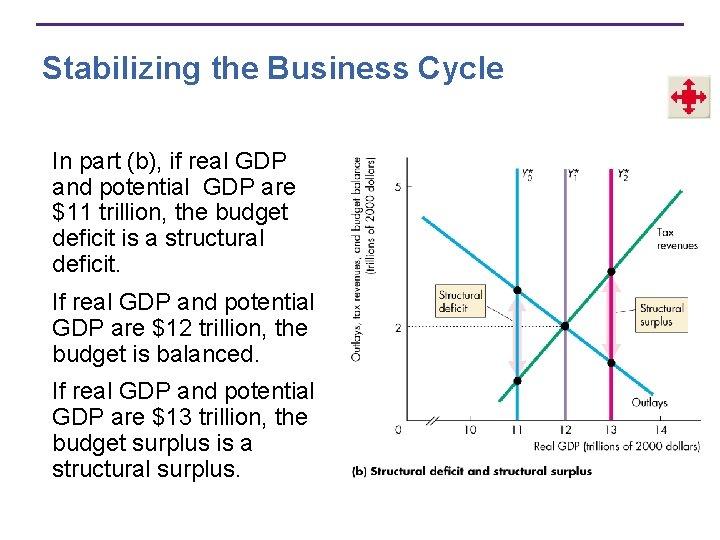
Stabilizing the Business Cycle In part (b), if real GDP and potential GDP are $11 trillion, the budget deficit is a structural deficit. If real GDP and potential GDP are $12 trillion, the budget is balanced. If real GDP and potential GDP are $13 trillion, the budget surplus is a structural surplus.

THE END