Chapter Eleven Monopoly Topics Monopoly Profit Maximization Effects

Chapter Eleven Monopoly

Topics § § § § Monopoly Profit Maximization. Effects of a Shift of the Demand Curve. Market Power. Welfare Effects of Monopoly. Cost Advantages That Create Monopolies. Government Actions That Reduce Market Power. Network Externalities, Behavioral Economics, and Monopoly Decisions over Time. © 2009 Pearson Addison-Wesley. All rights reserved. 2

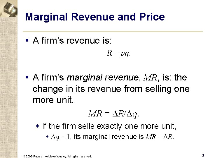
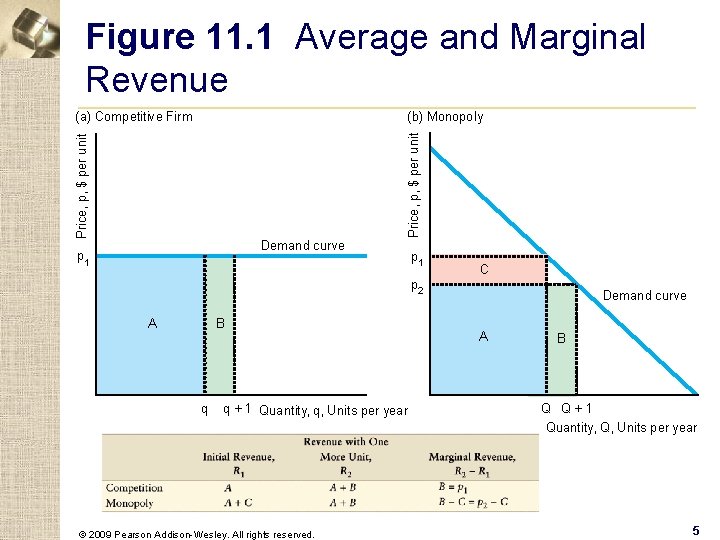
Marginal Revenue and Price § A firm’s revenue is: R = pq. § A firm’s marginal revenue, MR, is: the change in its revenue from selling one more unit. MR = ΔR/Δq. w If the firm sells exactly one more unit, Δq = 1, its marginal revenue is MR = ΔR. © 2009 Pearson Addison-Wesley. All rights reserved. 3

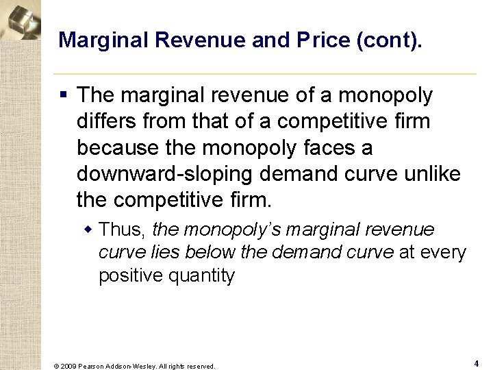
Marginal Revenue and Price (cont). § The marginal revenue of a monopoly differs from that of a competitive firm because the monopoly faces a downward-sloping demand curve unlike the competitive firm. w Thus, the monopoly’s marginal revenue curve lies below the demand curve at every positive quantity © 2009 Pearson Addison-Wesley. All rights reserved. 4

Figure 11. 1 Average and Marginal Revenue (b) Monopoly Price, p, $ per unit (a) Competitive Firm Demand curve p 1 C p 2 A B q q + 1 Quantity, q, Units per year © 2009 Pearson Addison-Wesley. All rights reserved. Demand curve A B Q Q+1 Quantity, Q, Units per year 5

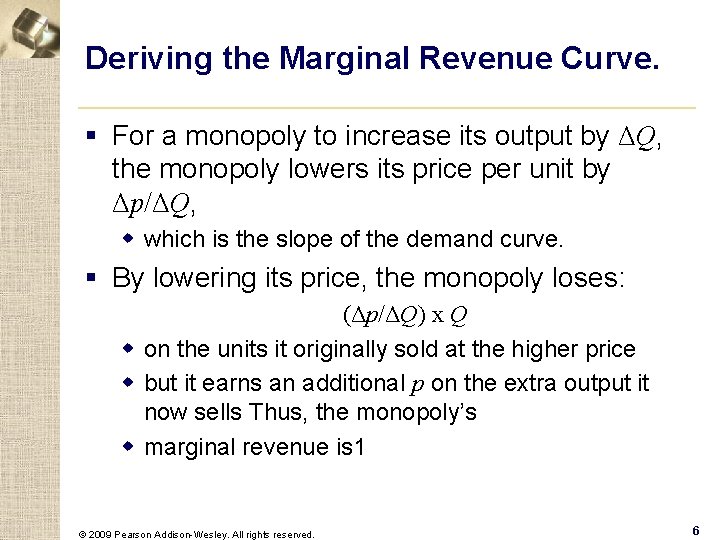
Deriving the Marginal Revenue Curve. § For a monopoly to increase its output by ΔQ, the monopoly lowers its price per unit by Δp/ΔQ, w which is the slope of the demand curve. § By lowering its price, the monopoly loses: (Δp/ΔQ) x Q w on the units it originally sold at the higher price w but it earns an additional p on the extra output it now sells Thus, the monopoly’s w marginal revenue is 1 © 2009 Pearson Addison-Wesley. All rights reserved. 6

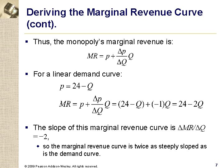
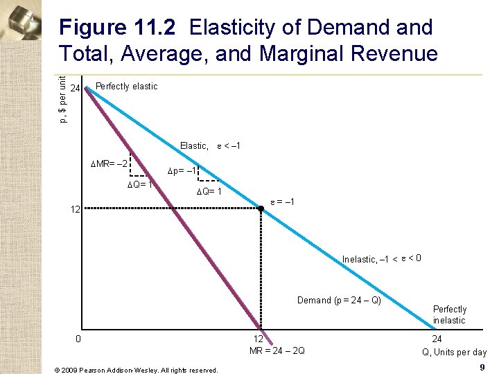
Deriving the Marginal Revenue Curve (cont). § Thus, the monopoly’s marginal revenue is: § For a linear demand curve: § The slope of this marginal revenue curve is ΔMR/ΔQ = − 2, w so the marginal revenue curve is twice as steeply sloped as is the demand curve. © 2009 Pearson Addison-Wesley. All rights reserved. 7

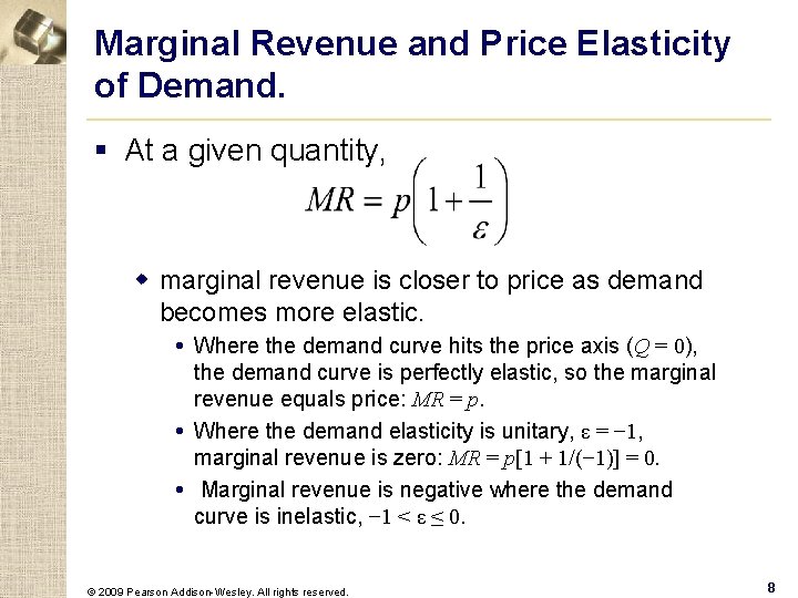
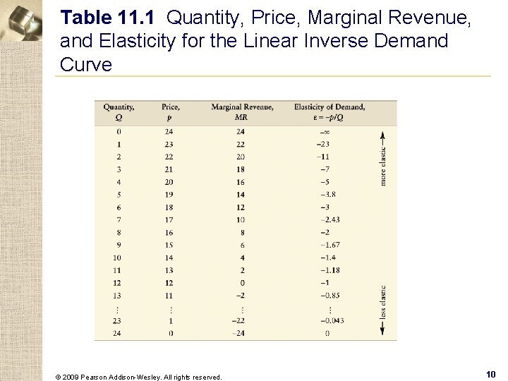
Marginal Revenue and Price Elasticity of Demand. § At a given quantity, w marginal revenue is closer to price as demand becomes more elastic. Where the demand curve hits the price axis (Q = 0), the demand curve is perfectly elastic, so the marginal revenue equals price: MR = p. Where the demand elasticity is unitary, ε = − 1, marginal revenue is zero: MR = p[1 + 1/(− 1)] = 0. Marginal revenue is negative where the demand curve is inelastic, − 1 < ε ≤ 0. © 2009 Pearson Addison-Wesley. All rights reserved. 8

p, $ per unit Figure 11. 2 Elasticity of Demand Total, Average, and Marginal Revenue 24 Perfectly elastic Elastic, e < – 1 DMR= – 2 Dp = – 1 DQ = 1 DQ= 1 12 e = – 1 Inelastic, – 1 < e < 0 Demand (p = 24 – Q) 0 © 2009 Pearson Addison-Wesley. All rights reserved. 12 MR = 24 – 2 Q Perfectly inelastic 24 Q, Units per day 9

Table 11. 1 Quantity, Price, Marginal Revenue, and Elasticity for the Linear Inverse Demand Curve © 2009 Pearson Addison-Wesley. All rights reserved. 10

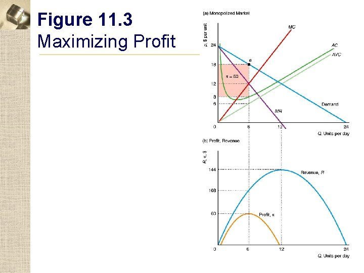
Figure 11. 3 Maximizing Profit

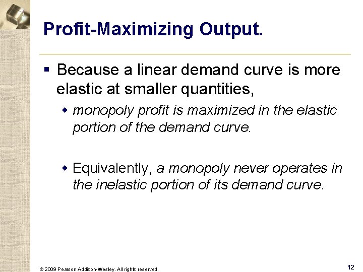
Profit-Maximizing Output. § Because a linear demand curve is more elastic at smaller quantities, w monopoly profit is maximized in the elastic portion of the demand curve. w Equivalently, a monopoly never operates in the inelastic portion of its demand curve. © 2009 Pearson Addison-Wesley. All rights reserved. 12

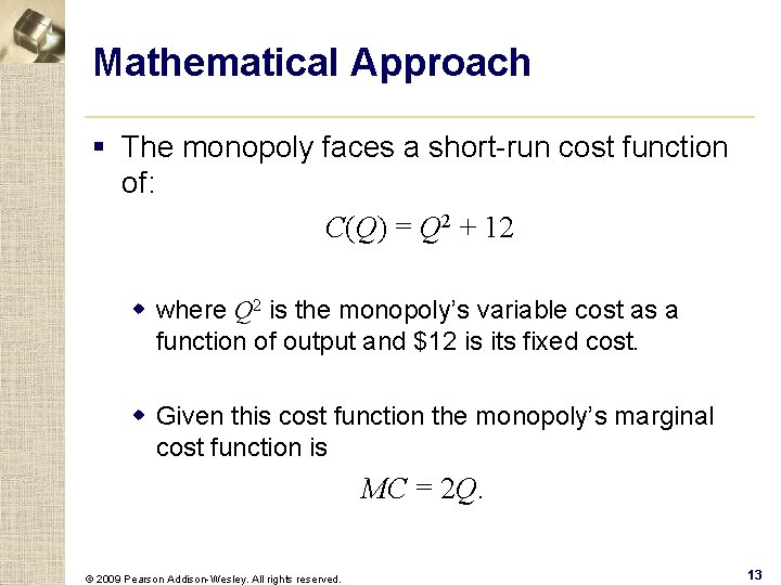
Mathematical Approach § The monopoly faces a short-run cost function of: C(Q) = Q 2 + 12 w where Q 2 is the monopoly’s variable cost as a function of output and $12 is its fixed cost. w Given this cost function the monopoly’s marginal cost function is MC = 2 Q. © 2009 Pearson Addison-Wesley. All rights reserved. 13

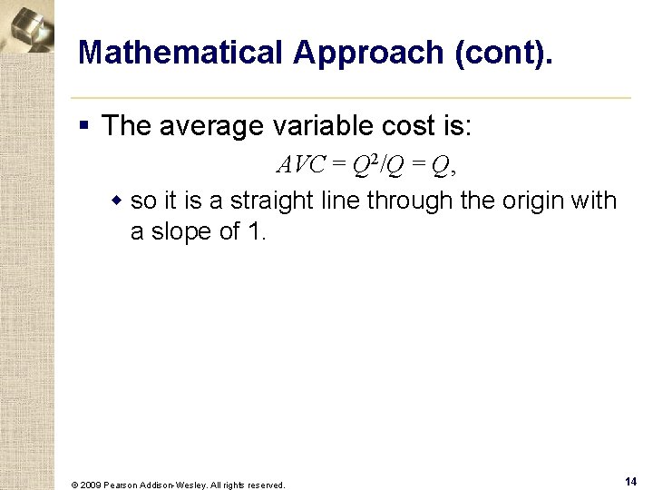
Mathematical Approach (cont). § The average variable cost is: AVC = Q 2/Q = Q, w so it is a straight line through the origin with a slope of 1. © 2009 Pearson Addison-Wesley. All rights reserved. 14

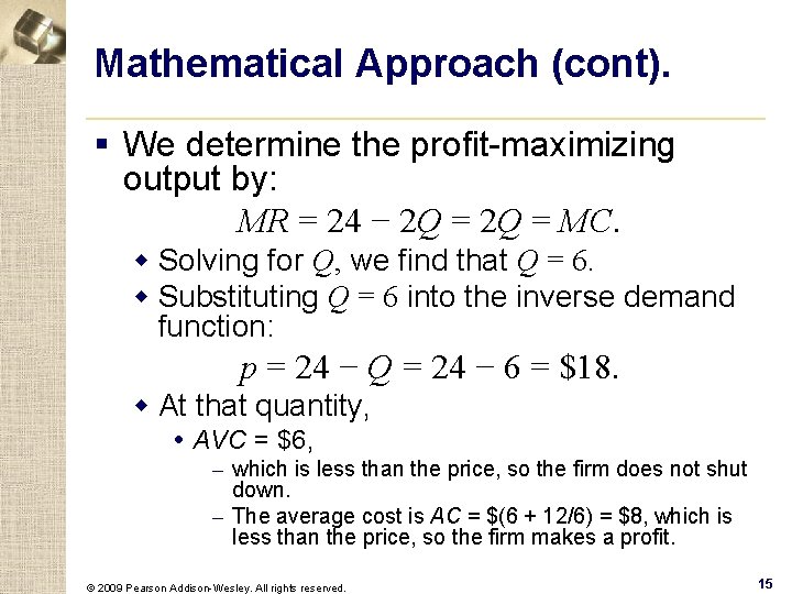
Mathematical Approach (cont). § We determine the profit-maximizing output by: MR = 24 − 2 Q = MC. w Solving for Q, we find that Q = 6. w Substituting Q = 6 into the inverse demand function: p = 24 − Q = 24 − 6 = $18. w At that quantity, AVC = $6, – which is less than the price, so the firm does not shut down. – The average cost is AC = $(6 + 12/6) = $8, which is less than the price, so the firm makes a profit. © 2009 Pearson Addison-Wesley. All rights reserved. 15

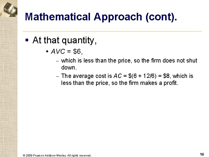
Mathematical Approach (cont). § At that quantity, AVC = $6, – which is less than the price, so the firm does not shut down. – The average cost is AC = $(6 + 12/6) = $8, which is less than the price, so the firm makes a profit. © 2009 Pearson Addison-Wesley. All rights reserved. 16

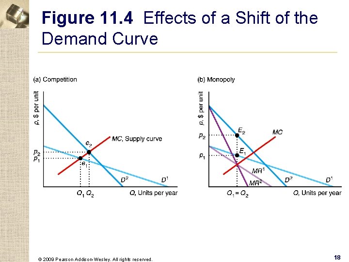
Effects of a Shift of the Demand Curve § Unlike a competitive firm, a monopoly does not have a supply curve. § A given quantity can correspond to more than one monopoly-optimal price. w A shift in the demand curve may cause the monopoly optimal price to stay constant and the quantity to change or both price and quantity to change. © 2009 Pearson Addison-Wesley. All rights reserved. 17

Figure 11. 4 Effects of a Shift of the Demand Curve © 2009 Pearson Addison-Wesley. All rights reserved. 18

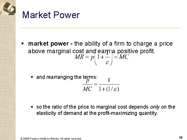
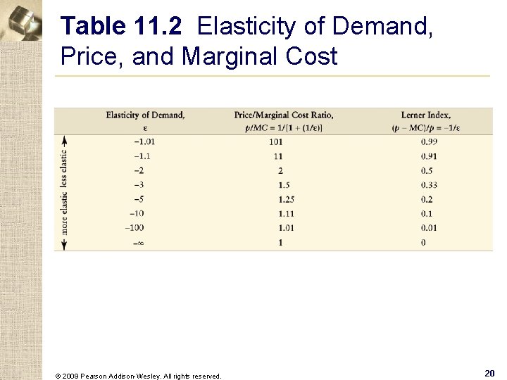
Market Power § market power - the ability of a firm to charge a price above marginal cost and earn a positive profit. w and rearranging the terms: w so the ratio of the price to marginal cost depends only on the elasticity of demand at the profit-maximizing quantity. © 2009 Pearson Addison-Wesley. All rights reserved. 19

Table 11. 2 Elasticity of Demand, Price, and Marginal Cost © 2009 Pearson Addison-Wesley. All rights reserved. 20

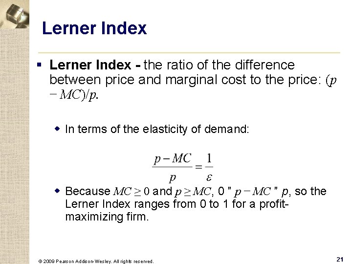
Lerner Index § Lerner Index - the ratio of the difference between price and marginal cost to the price: (p − MC)/p. w In terms of the elasticity of demand: w Because MC ≥ 0 and p ≥ MC, 0 ″ p − MC ″ p, so the Lerner Index ranges from 0 to 1 for a profitmaximizing firm. © 2009 Pearson Addison-Wesley. All rights reserved. 21

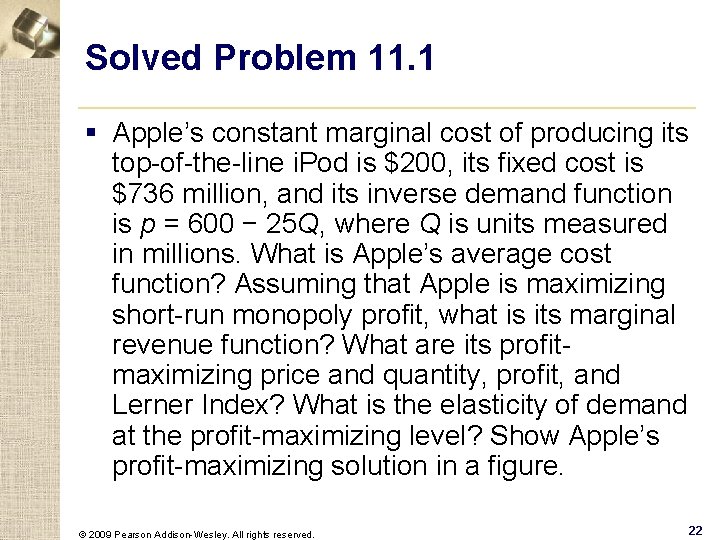
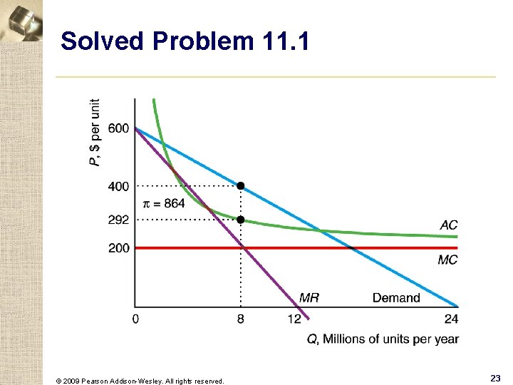
Solved Problem 11. 1 § Apple’s constant marginal cost of producing its top-of-the-line i. Pod is $200, its fixed cost is $736 million, and its inverse demand function is p = 600 − 25 Q, where Q is units measured in millions. What is Apple’s average cost function? Assuming that Apple is maximizing short-run monopoly profit, what is its marginal revenue function? What are its profitmaximizing price and quantity, profit, and Lerner Index? What is the elasticity of demand at the profit-maximizing level? Show Apple’s profit-maximizing solution in a figure. © 2009 Pearson Addison-Wesley. All rights reserved. 22

Solved Problem 11. 1 © 2009 Pearson Addison-Wesley. All rights reserved. 23

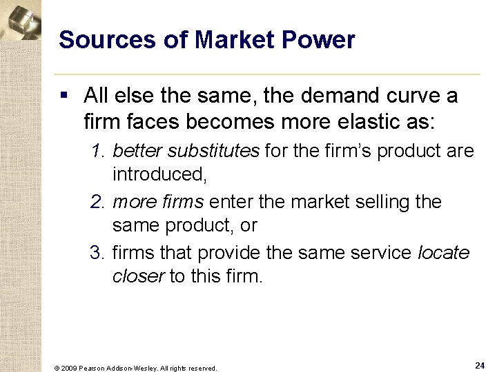
Sources of Market Power § All else the same, the demand curve a firm faces becomes more elastic as: 1. better substitutes for the firm’s product are introduced, 2. more firms enter the market selling the same product, or 3. firms that provide the same service locate closer to this firm. © 2009 Pearson Addison-Wesley. All rights reserved. 24

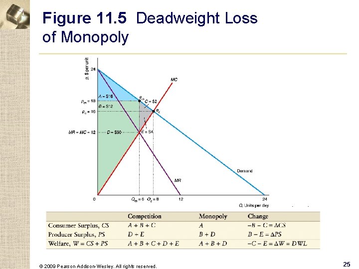
Figure 11. 5 Deadweight Loss of Monopoly © 2009 Pearson Addison-Wesley. All rights reserved. 25

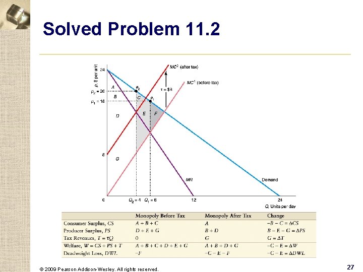
Solved Problem 11. 2 § In the linear example in Figure 11. 3, how does charging the monopoly a specific tax of τ = $8 per unit affect the monopoly optimum and the welfare of consumers, the monopoly, and society (where society’s welfare includes the tax revenue)? What is the incidence of the tax on consumers? © 2009 Pearson Addison-Wesley. All rights reserved. 26

Solved Problem 11. 2 © 2009 Pearson Addison-Wesley. All rights reserved. 27

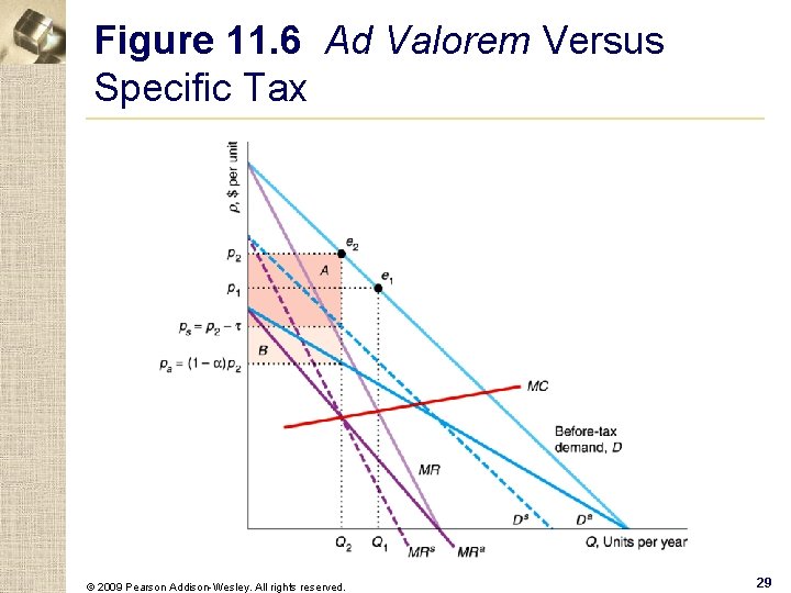
Welfare Effects of Ad Valorem Versus Specific Taxes § A government raises more tax revenue with an ad valorem tax applied to a monopoly than with a specific tax when α and τ are set so that the after-tax output is the same with either tax. © 2009 Pearson Addison-Wesley. All rights reserved. 28

Figure 11. 6 Ad Valorem Versus Specific Tax © 2009 Pearson Addison-Wesley. All rights reserved. 29

Cost Advantages That Create Monopolies § Why are some markets monopolized? w a firm has a cost advantage over other firms or w a government created the monopoly © 2009 Pearson Addison-Wesley. All rights reserved. 30

Sources of Cost Advantages § Reasons for cost advantages: w the firm controls an essential facility: a scarce resource that a rival needs to use to survive. w the firm uses a superior technology or has a better way of organizing production © 2009 Pearson Addison-Wesley. All rights reserved. 31

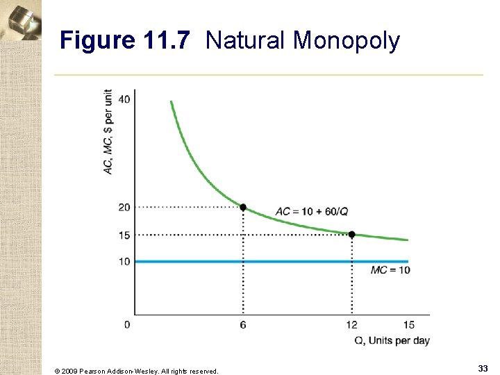
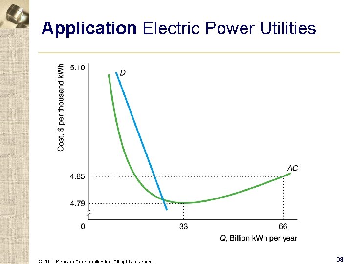
Natural Monopoly § natural monopoly - situation in which one firm can produce the total output of the market at lower cost than several firms could. § Believing that they are natural monopolies, governments frequently grant monopoly rights to public utilities to provide essential goods or services such as water, gas, electric power, or mail delivery © 2009 Pearson Addison-Wesley. All rights reserved. 32

Figure 11. 7 Natural Monopoly © 2009 Pearson Addison-Wesley. All rights reserved. 33

Solved Problem 11. 3 § A firm that delivers Q units of water to households has a total cost of C(Q) = m. Q + F. If any entrant would have the same cost, does this market have a natural monopoly? © 2009 Pearson Addison-Wesley. All rights reserved. 34

Government Actions That Create Monopolies § Governments create many monopolies. w Sometimes governments own and manage monopolies. w In the United States, as in most countries, the postal service is a government monopoly. § Frequently, however, governments create monopolies by preventing competing firms from entering a market. © 2009 Pearson Addison-Wesley. All rights reserved. 35

Barriers to Entry § Governments create monopolies in one of three ways: 1. by making it difficult for new firms to obtain a license to operate, 2. by granting a firm the rights to be a monopoly, or 3. by auctioning the rights to be monopoly. © 2009 Pearson Addison-Wesley. All rights reserved. 36

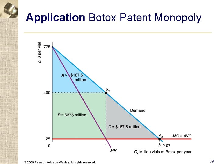
Patents § Patent - an exclusive right granted to the inventor to sell a new and useful product, process, substance, or design for a fixed period of time. w The length of a patent varies across countries. § Question: If a firm with a patent monopoly sets a high price that results in deadweight loss then why do governments grant patent monopolies? © 2009 Pearson Addison-Wesley. All rights reserved. 37

Application Electric Power Utilities © 2009 Pearson Addison-Wesley. All rights reserved. 38

Application Botox Patent Monopoly © 2009 Pearson Addison-Wesley. All rights reserved. 39

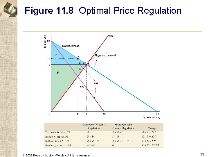
Optimal Price Regulation § In some markets, the government can eliminate the deadweight loss of monopoly by requiring that a monopoly charge no more than the competitive price. © 2009 Pearson Addison-Wesley. All rights reserved. 40

Figure 11. 8 Optimal Price Regulation © 2009 Pearson Addison-Wesley. All rights reserved. 41

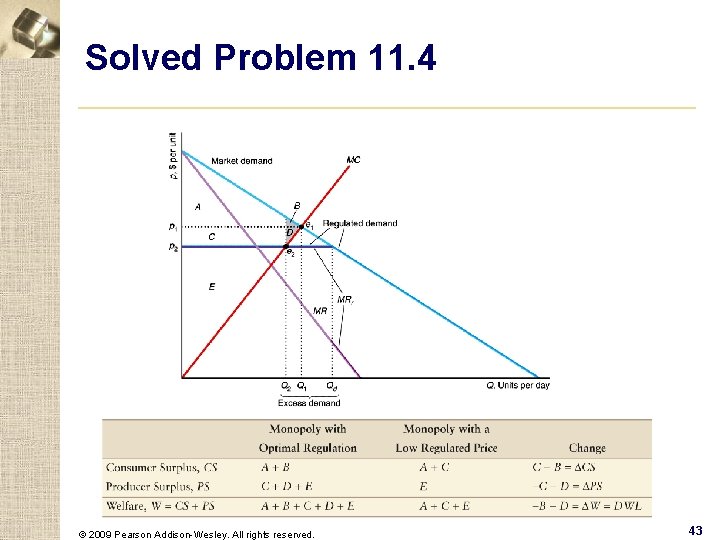
Solved Problem 11. 4 § Suppose that the government sets a price, p 2, that is below the socially optimal level, p 1, but above the monopoly’s minimum average cost. How do the price, the quantity sold, the quantity demanded, and welfare under this regulation compare to those under optimal regulation? © 2009 Pearson Addison-Wesley. All rights reserved. 42

Solved Problem 11. 4 © 2009 Pearson Addison-Wesley. All rights reserved. 43

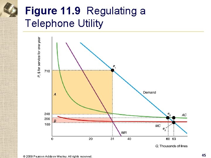
Problems in Regulating § Problems that governments face in regulating monopolies: w because they do not know the actual demand marginal cost curves, governments may set the price at the wrong level. w Second, many governments use regulations that are less efficient than price regulation. w Third, regulated firms may bribe or otherwise influence government regulators to help the firms rather than society as a whole. © 2009 Pearson Addison-Wesley. All rights reserved. 44

Figure 11. 9 Regulating a Telephone Utility © 2009 Pearson Addison-Wesley. All rights reserved. 45

Increasing Competition § Encouraging competition is an alternative to regulation as a means of reducing the harms of monopoly. © 2009 Pearson Addison-Wesley. All rights reserved. 46

Network Externalities § network externality - the situation where one person’s demand for a good depends on the consumption of the good by others © 2009 Pearson Addison-Wesley. All rights reserved. 47

Direct Size Effect. § Many industries exhibit positive network externalities where the customer gets a direct benefit from a larger network. w Example: the larger an ATM network such as the Plus network © 2009 Pearson Addison-Wesley. All rights reserved. 48

Behavioral Economics. § bandwagon effect - the situation in which a person places greater value on a good as more and more other people possess it § snob effect - the situation in which a person places greater value on a good as fewer and fewer other people possess it © 2009 Pearson Addison-Wesley. All rights reserved. 49