Chapter Eight Competitive Firms and Markets Topics Competition

Chapter Eight Competitive Firms and Markets

Topics § Competition. § Profit Maximization. § Competition in the Short Run. § Competition in the Long Run. § Zero Profit for Competitive Firms in the Long Run. © 2009 Pearson Addison-Wesley. All rights reserved. 2

Price Taking § A market is competitive if each firm in the market is a price taker. w price taker - a firm that cannot significantly affect the market price for its output or the prices at which it buys its inputs. w the price taker firm faces a demand curve that is horizontal at the market price. © 2009 Pearson Addison-Wesley. All rights reserved. 3

Why the Firm’s Demand Curve Is Horizontal § Consumers believe that all firms in the market sell identical products. § Firms freely enter and exit the market. § Buyers and sellers know the prices charged by firms. § Transaction costs are low. We call a market in which all these conditions hold a perfectly competitive market. © 2009 Pearson Addison-Wesley. All rights reserved. 4

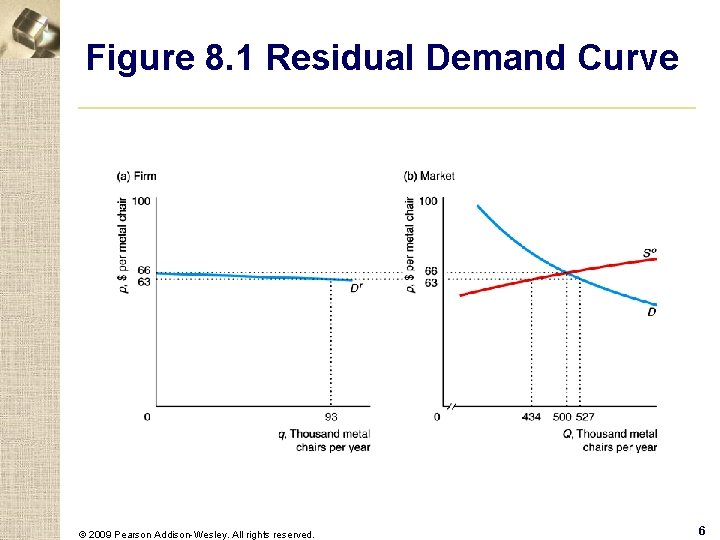
Derivation of a Competitive Firm’s Demand Curve § residual demand curve - the market demand that is not met by other sellers at any given price. D’(p) = D(p) − So(p). © 2009 Pearson Addison-Wesley. All rights reserved. 5

Figure 8. 1 Residual Demand Curve © 2009 Pearson Addison-Wesley. All rights reserved. 6

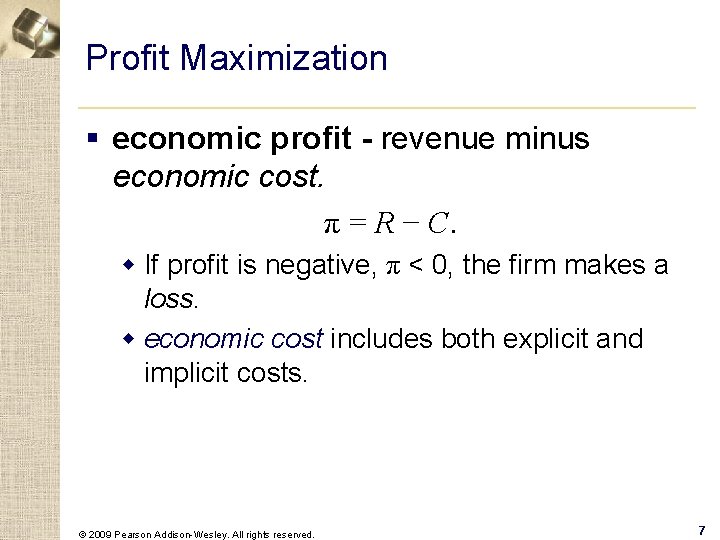
Profit Maximization § economic profit - revenue minus economic cost. π = R − C. w If profit is negative, π < 0, the firm makes a loss. w economic cost includes both explicit and implicit costs. © 2009 Pearson Addison-Wesley. All rights reserved. 7

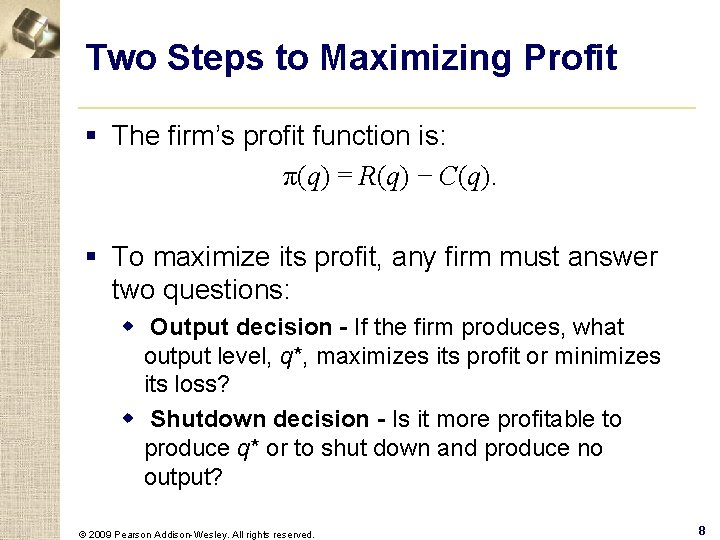
Two Steps to Maximizing Profit § The firm’s profit function is: π(q) = R(q) − C(q). § To maximize its profit, any firm must answer two questions: w Output decision - If the firm produces, what output level, q*, maximizes its profit or minimizes its loss? w Shutdown decision - Is it more profitable to produce q* or to shut down and produce no output? © 2009 Pearson Addison-Wesley. All rights reserved. 8

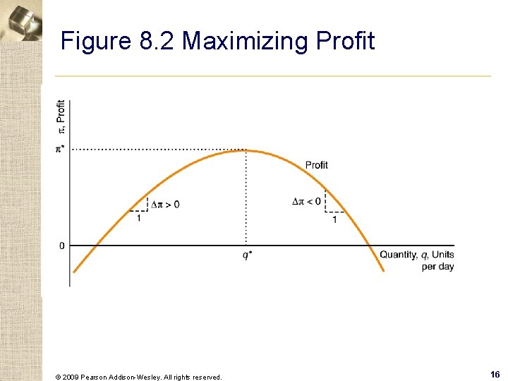
Output Rules. § Output Rule 1: The firm sets its output where its profit is maximized. § Output Rule 2: A firm sets its output where its marginal profit is zero. © 2009 Pearson Addison-Wesley. All rights reserved. 9

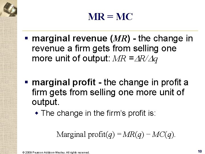
MR = MC § marginal revenue (MR) - the change in revenue a firm gets from selling one more unit of output: MR =DR/Dq § marginal profit - the change in profit a firm gets from selling one more unit of output. w The change in the firm’s profit is: Marginal profit(q) = MR(q) − MC(q). © 2009 Pearson Addison-Wesley. All rights reserved. 10

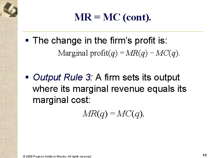
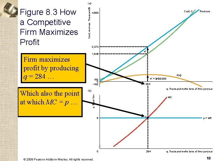
MR = MC (cont). § The change in the firm’s profit is: Marginal profit(q) = MR(q) − MC(q). § Output Rule 3: A firm sets its output where its marginal revenue equals its marginal cost: MR(q) = MC(q). © 2009 Pearson Addison-Wesley. All rights reserved. 11

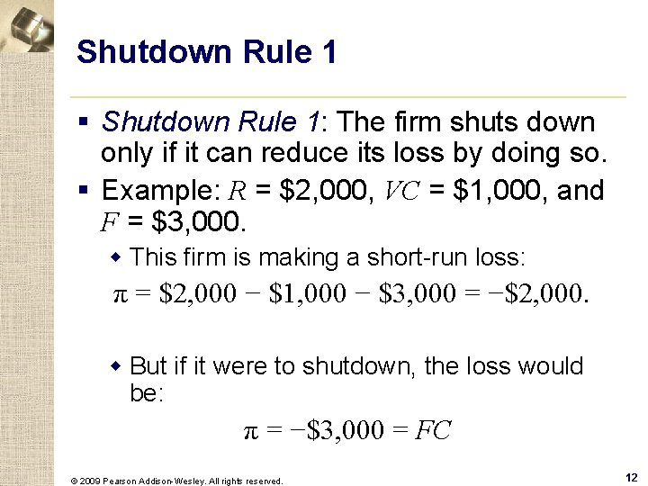
Shutdown Rule 1 § Shutdown Rule 1: The firm shuts down only if it can reduce its loss by doing so. § Example: R = $2, 000, VC = $1, 000, and F = $3, 000. w This firm is making a short-run loss: π = $2, 000 − $1, 000 − $3, 000 = −$2, 000. w But if it were to shutdown, the loss would be: π = −$3, 000 = FC © 2009 Pearson Addison-Wesley. All rights reserved. 12

Shutdown Rule 2 § Shutdown Rule 2: The firm shuts down only if its revenue is less than its avoidable cost. © 2009 Pearson Addison-Wesley. All rights reserved. 13

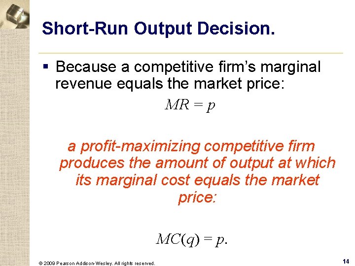
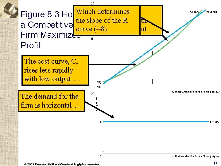
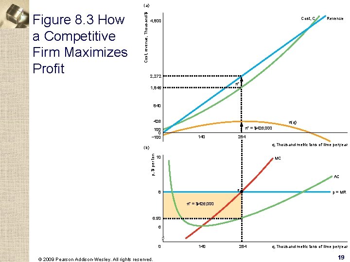
Short-Run Output Decision. § Because a competitive firm’s marginal revenue equals the market price: MR = p a profit-maximizing competitive firm produces the amount of output at which its marginal cost equals the market price: MC(q) = p. © 2009 Pearson Addison-Wesley. All rights reserved. 14

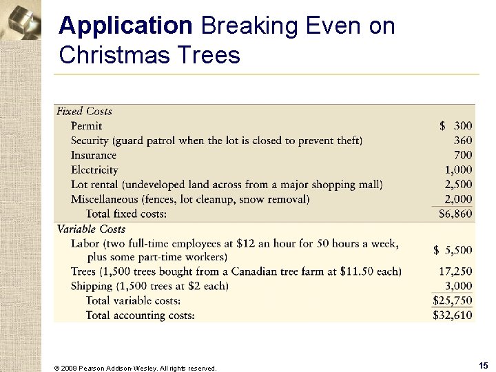
Application Breaking Even on Christmas Trees © 2009 Pearson Addison-Wesley. All rights reserved. 15

Figure 8. 2 Maximizing Profit © 2009 Pearson Addison-Wesley. All rights reserved. 16

(a) The cost curve, C, rises less rapidly with low output…. The demand for the firm is horizontal…. 4, 800 Cost, C Revenue 100 0 100 q, Thousand metric tons of lime peryear (b) p, $ per ton Firm Maximizes Profit Cost, revenue, Thousand $ and more Figure 8. 3 How. Which determines the slope of rapidly the R with a Competitive curve (=8) more output. 8 p = MR 0 q, Thousand metric tons of lime peryear © 2009 Pearson Addison-Wesley. All rights reserved. Pearson Addison-Wesley. rights reserved. 17

Revenue 2, 272 1, 846 Firm maximizes profit by producing q = 284 … Which also the point at which MC = p … Cost, C 4, 800 p* p(q) 100 0 – 100 p* = $426, 000 284 q, Thousand metric tons of lime peryear (b) p, $ per ton Figure 8. 3 How a Competitive Firm Maximizes Profit Cost, revenue, Thousand $ (a) MC 8 0 © 2009 Pearson Addison-Wesley. All rights reserved. e 284 p = MR q, Thousand metric tons of lime peryear 18

Figure 8. 3 How a Competitive Firm Maximizes Profit Cost, revenue, Thousand $ (a) Cost, C 4, 800 Revenue 2, 272 p* 1, 846 840 426 100 0 – 100 p(q) p* = $426, 000 140 284 q, Thousand metric tons of lime peryear p, $ per ton (b) 10 MC AC e 8 p = MR p* = $426, 000 6. 50 6 0 © 2009 Pearson Addison-Wesley. All rights reserved. 140 284 q, Thousand metric tons of lime peryear 19

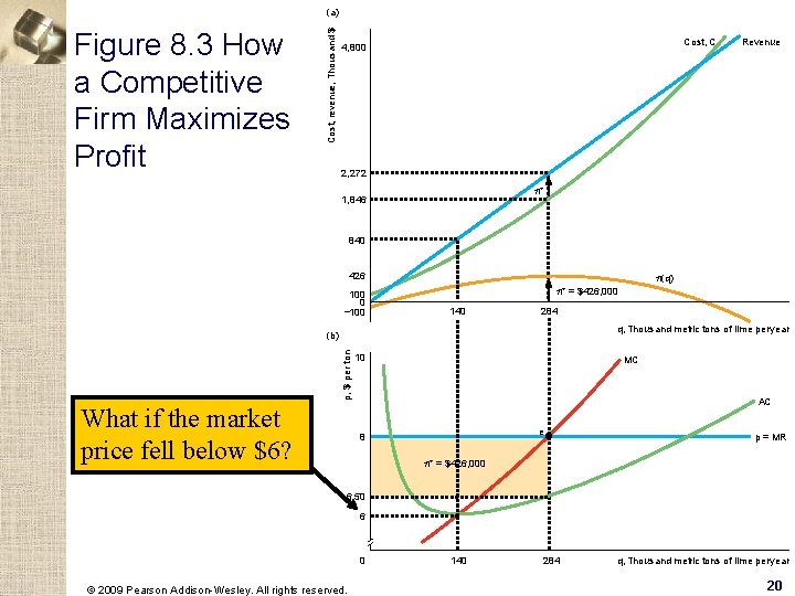
Figure 8. 3 How a Competitive Firm Maximizes Profit Cost, revenue, Thousand $ (a) Cost, C 4, 800 Revenue 2, 272 p* 1, 846 840 426 100 0 – 100 p(q) p* = $426, 000 140 284 q, Thousand metric tons of lime peryear p, $ per ton (b) What if the market price fell below $6? 10 MC AC e 8 p = MR p* = $426, 000 6. 50 6 0 © 2009 Pearson Addison-Wesley. All rights reserved. 140 284 q, Thousand metric tons of lime peryear 20

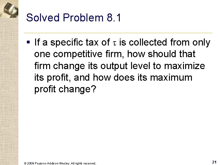
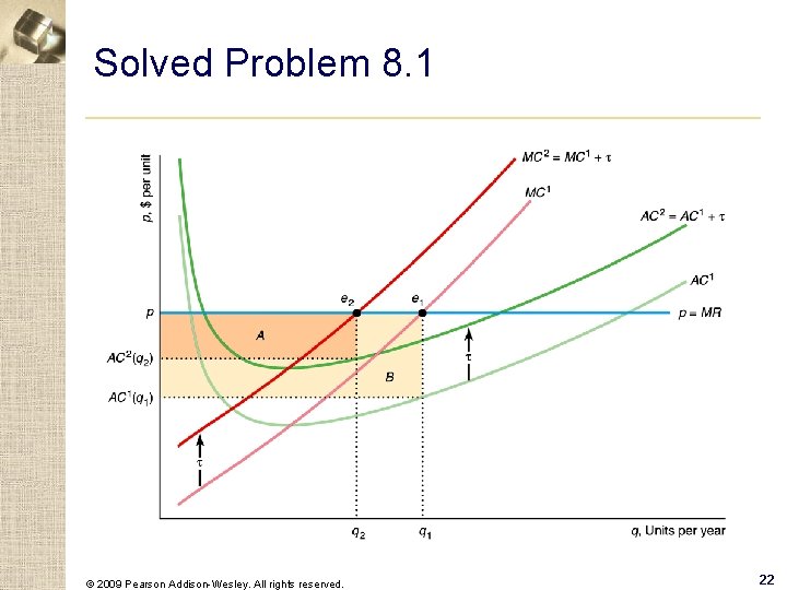
Solved Problem 8. 1 § If a specific tax of τ is collected from only one competitive firm, how should that firm change its output level to maximize its profit, and how does its maximum profit change? © 2009 Pearson Addison-Wesley. All rights reserved. 21

Solved Problem 8. 1 © 2009 Pearson Addison-Wesley. All rights reserved. 22

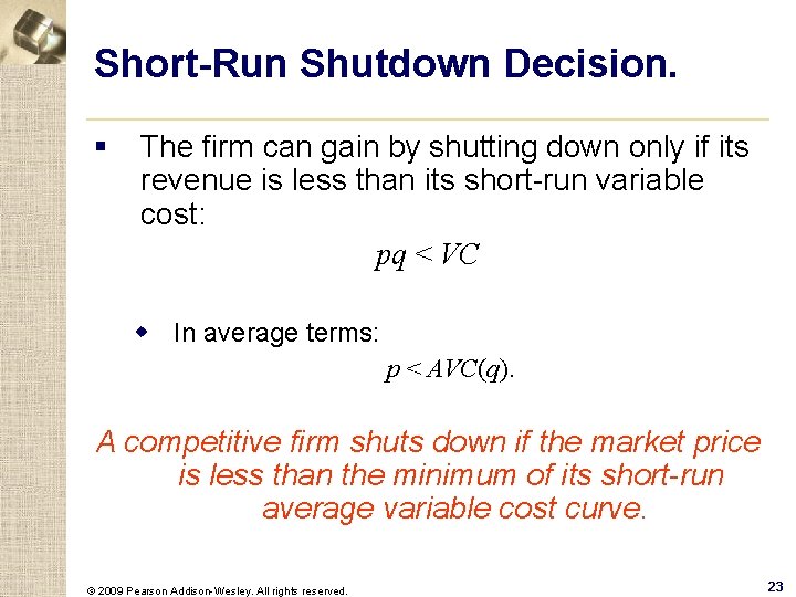
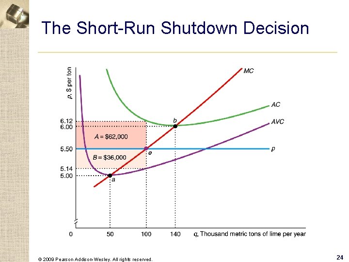
Short-Run Shutdown Decision. § The firm can gain by shutting down only if its revenue is less than its short-run variable cost: pq < VC w In average terms: p < AVC(q). A competitive firm shuts down if the market price is less than the minimum of its short-run average variable cost curve. © 2009 Pearson Addison-Wesley. All rights reserved. 23

The Short-Run Shutdown Decision © 2009 Pearson Addison-Wesley. All rights reserved. 24

Solved Problem 8. 2 § A competitive firm’s bookkeeper, upon reviewing the firm’s books, finds that the firm spent twice as much on its plant, a fixed cost, as the firm’s manager had previously thought. Should the manager change the output level because of this new information? How does this new information affect profit? © 2009 Pearson Addison-Wesley. All rights reserved. 25

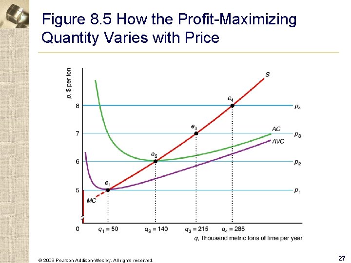
Short-Run Firm Supply Curve § If the price falls below the firm’s minimum average variable cost the firm shuts down. w Thus: the competitive firm’s short-run supply curve is its marginal cost curve above its minimum average variable cost. © 2009 Pearson Addison-Wesley. All rights reserved. 26

Figure 8. 5 How the Profit-Maximizing Quantity Varies with Price © 2009 Pearson Addison-Wesley. All rights reserved. 27

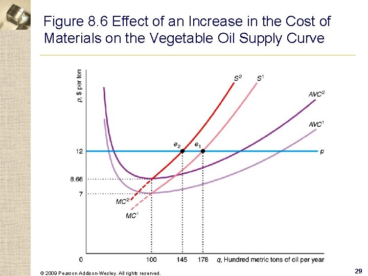
Factor Prices and the Short-Run Firm Supply Curve § An increase in factor prices causes the production costs of a firm to rise, shifting the firm’s supply curve to the left. © 2009 Pearson Addison-Wesley. All rights reserved. 28

Figure 8. 6 Effect of an Increase in the Cost of Materials on the Vegetable Oil Supply Curve © 2009 Pearson Addison-Wesley. All rights reserved. 29

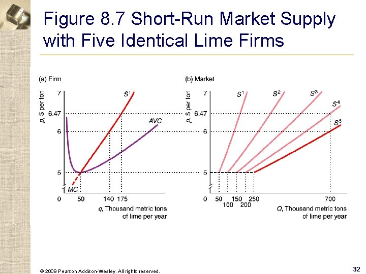
Short-Run Market Supply Curve § In the short run, the maximum number of firms in a market, n, is fixed. § If all the firms in a competitive market are identical, each firm’s supply curve is identical, so the market supply at any price is n times the supply of an individual firm. © 2009 Pearson Addison-Wesley. All rights reserved. 30

Short-Run Market Supply with Identical Firms. § As the number of firms grows very large, the market supply curve approaches a horizontal line at the minimum point of the AVC curve. § Thus, the more identical firms producing at a given price, the flatter (more elastic) the short-run market supply curve at that price © 2009 Pearson Addison-Wesley. All rights reserved. 31

Figure 8. 7 Short-Run Market Supply with Five Identical Lime Firms © 2009 Pearson Addison-Wesley. All rights reserved. 32

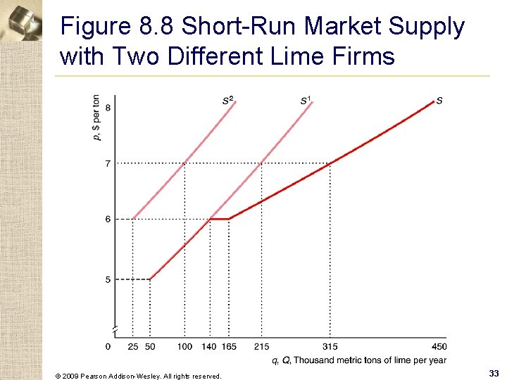
Figure 8. 8 Short-Run Market Supply with Two Different Lime Firms © 2009 Pearson Addison-Wesley. All rights reserved. 33

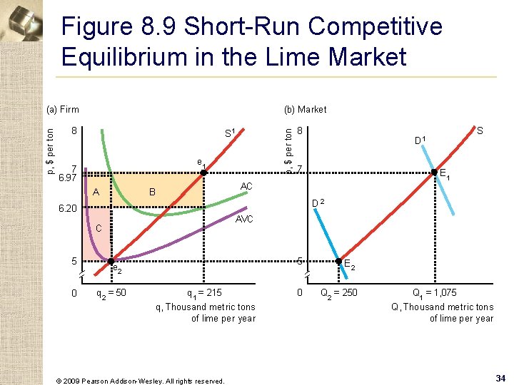
Figure 8. 9 Short-Run Competitive Equilibrium in the Lime Market (b) Market 8 S 1 p, $ per ton (a) Firm e 1 7 6. 97 A 8 7 D 2 6. 20 AVC C 5 0 E 1 AC B S D 1 5 e 2 q 2 = 50 q 1 = 215 q, Thousand metric tons of lime per year © 2009 Pearson Addison-Wesley. All rights reserved. 0 E 2 Q 2 = 250 Q 1 = 1, 075 Q, Thousand metric tons of lime per year 34

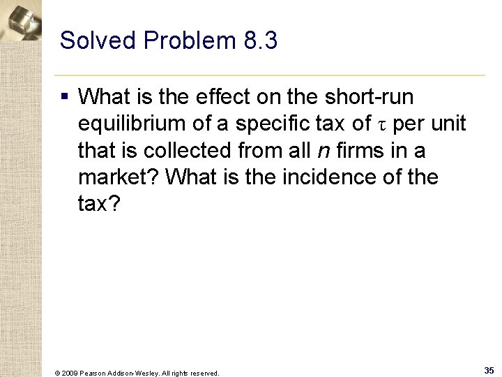
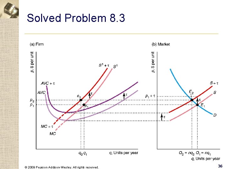
Solved Problem 8. 3 § What is the effect on the short-run equilibrium of a specific tax of τ per unit that is collected from all n firms in a market? What is the incidence of the tax? © 2009 Pearson Addison-Wesley. All rights reserved. 35

Solved Problem 8. 3 © 2009 Pearson Addison-Wesley. All rights reserved. 36

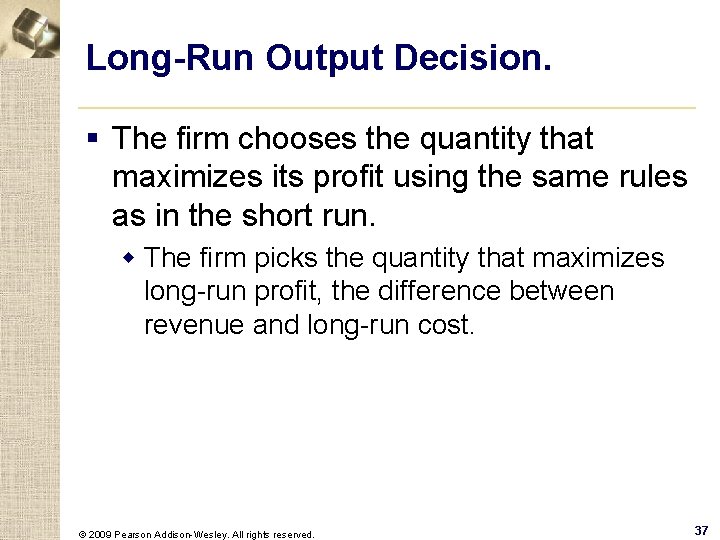
Long-Run Output Decision. § The firm chooses the quantity that maximizes its profit using the same rules as in the short run. w The firm picks the quantity that maximizes long-run profit, the difference between revenue and long-run cost. © 2009 Pearson Addison-Wesley. All rights reserved. 37

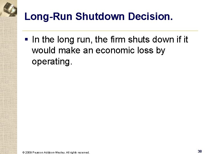
Long-Run Shutdown Decision. § In the long run, the firm shuts down if it would make an economic loss by operating. © 2009 Pearson Addison-Wesley. All rights reserved. 38

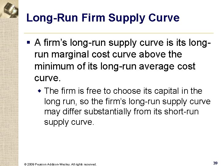
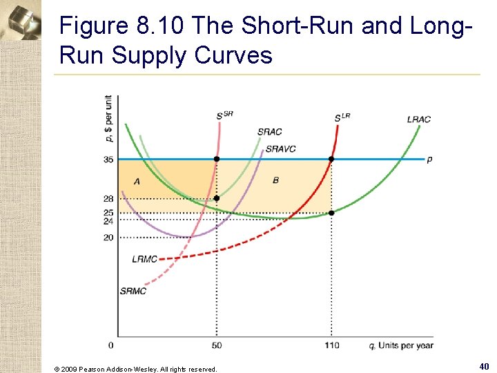
Long-Run Firm Supply Curve § A firm’s long-run supply curve is its longrun marginal cost curve above the minimum of its long-run average cost curve. w The firm is free to choose its capital in the long run, so the firm’s long-run supply curve may differ substantially from its short-run supply curve. © 2009 Pearson Addison-Wesley. All rights reserved. 39

Figure 8. 10 The Short-Run and Long. Run Supply Curves © 2009 Pearson Addison-Wesley. All rights reserved. 40

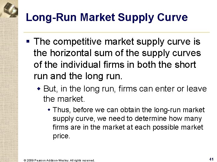
Long-Run Market Supply Curve § The competitive market supply curve is the horizontal sum of the supply curves of the individual firms in both the short run and the long run. w But, in the long run, firms can enter or leave the market. Thus, before we can obtain the long-run market supply curve, we need to determine how many firms are in the market at each possible market price. © 2009 Pearson Addison-Wesley. All rights reserved. 41

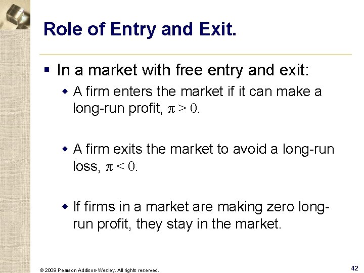
Role of Entry and Exit. § In a market with free entry and exit: w A firm enters the market if it can make a long-run profit, π > 0. w A firm exits the market to avoid a long-run loss, π < 0. w If firms in a market are making zero longrun profit, they stay in the market. © 2009 Pearson Addison-Wesley. All rights reserved. 42

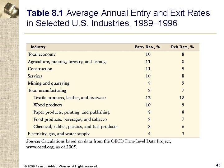
Table 8. 1 Average Annual Entry and Exit Rates in Selected U. S. Industries, 1989– 1996 © 2009 Pearson Addison-Wesley. All rights reserved. 43

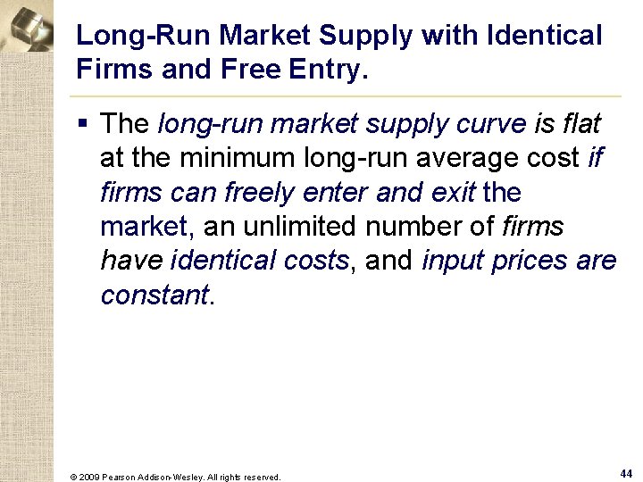
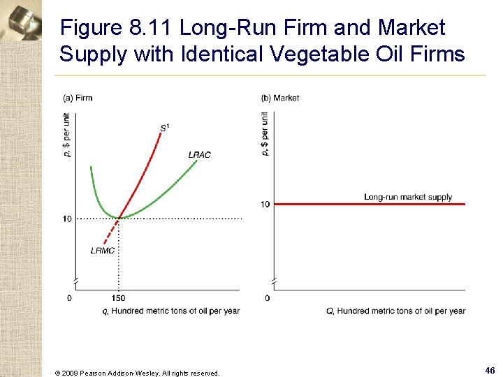
Long-Run Market Supply with Identical Firms and Free Entry. § The long-run market supply curve is flat at the minimum long-run average cost if firms can freely enter and exit the market, an unlimited number of firms have identical costs, and input prices are constant. © 2009 Pearson Addison-Wesley. All rights reserved. 44

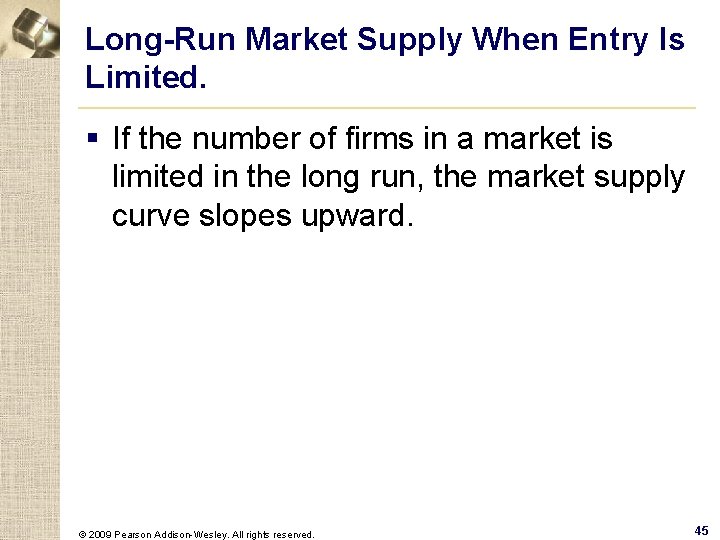
Long-Run Market Supply When Entry Is Limited. § If the number of firms in a market is limited in the long run, the market supply curve slopes upward. © 2009 Pearson Addison-Wesley. All rights reserved. 45

Figure 8. 11 Long-Run Firm and Market Supply with Identical Vegetable Oil Firms © 2009 Pearson Addison-Wesley. All rights reserved. 46

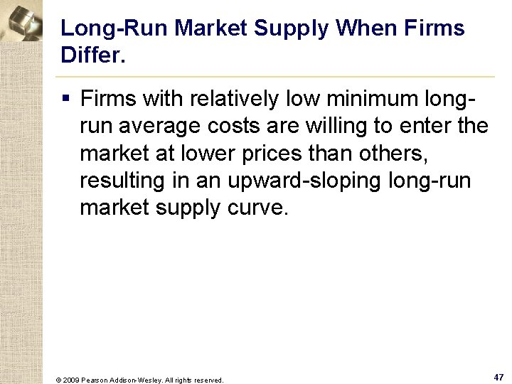
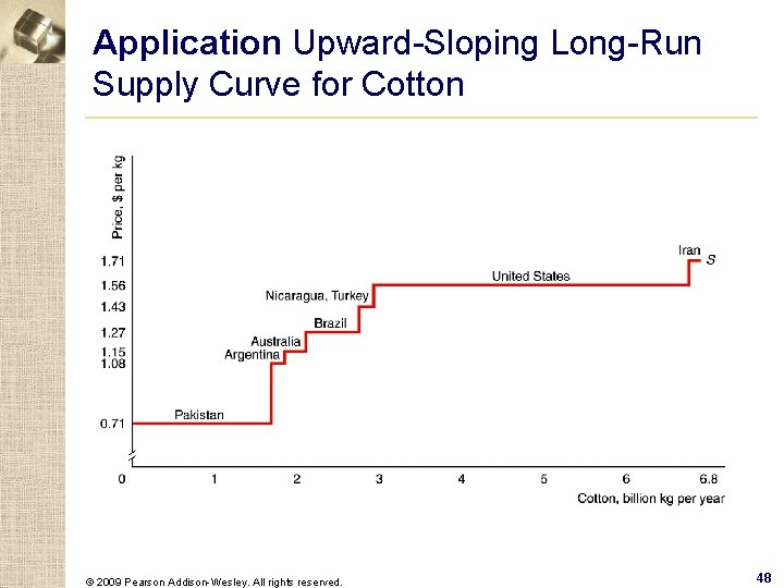
Long-Run Market Supply When Firms Differ. § Firms with relatively low minimum longrun average costs are willing to enter the market at lower prices than others, resulting in an upward-sloping long-run market supply curve. © 2009 Pearson Addison-Wesley. All rights reserved. 47

Application Upward-Sloping Long-Run Supply Curve for Cotton © 2009 Pearson Addison-Wesley. All rights reserved. 48

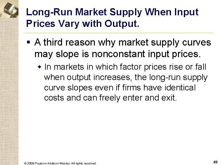
Long-Run Market Supply When Input Prices Vary with Output. § A third reason why market supply curves may slope is nonconstant input prices. w In markets in which factor prices rise or fall when output increases, the long-run supply curve slopes even if firms have identical costs and can freely enter and exit. © 2009 Pearson Addison-Wesley. All rights reserved. 49

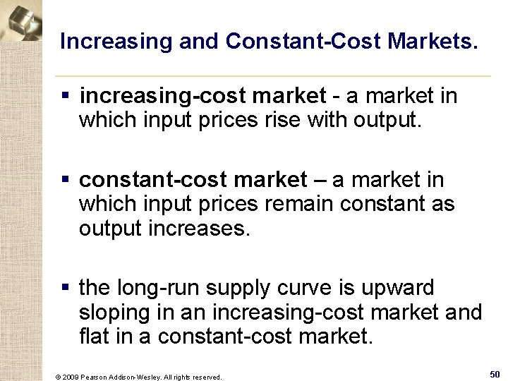
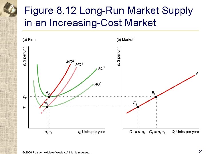
Increasing and Constant-Cost Markets. § increasing-cost market - a market in which input prices rise with output. § constant-cost market – a market in which input prices remain constant as output increases. § the long-run supply curve is upward sloping in an increasing-cost market and flat in a constant-cost market. © 2009 Pearson Addison-Wesley. All rights reserved. 50

Figure 8. 12 Long-Run Market Supply in an Increasing-Cost Market © 2009 Pearson Addison-Wesley. All rights reserved. 51

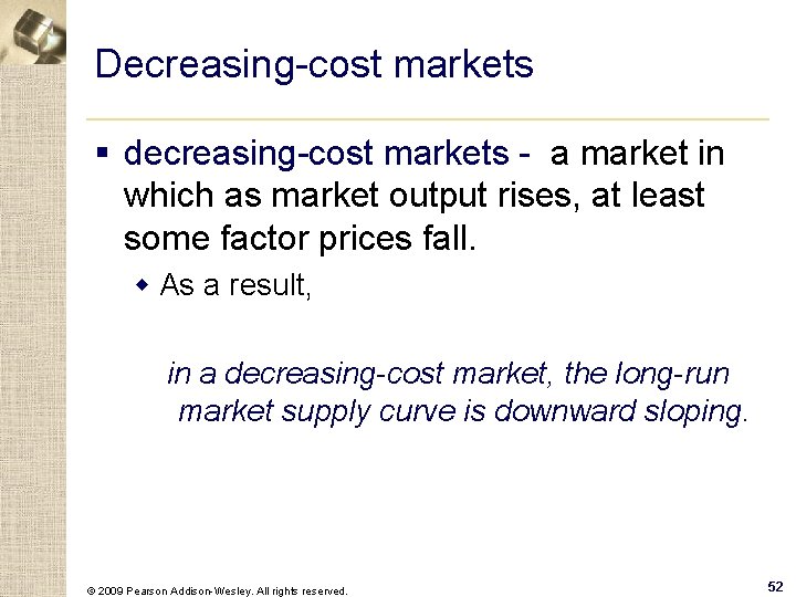
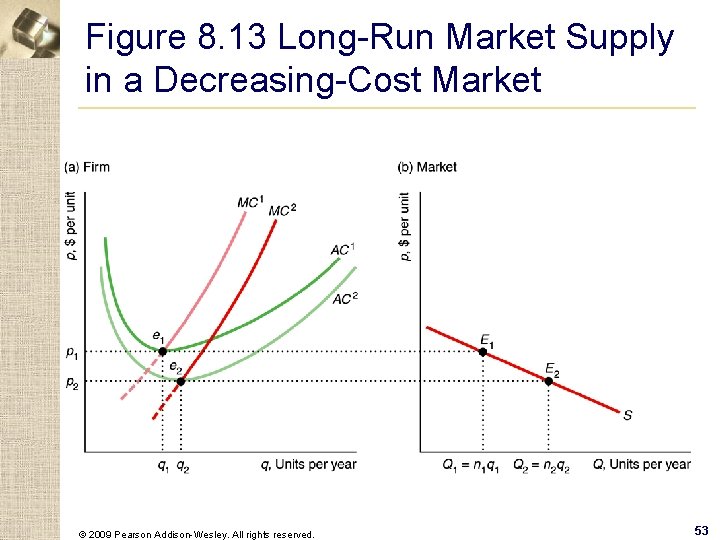
Decreasing-cost markets § decreasing-cost markets - a market in which as market output rises, at least some factor prices fall. w As a result, in a decreasing-cost market, the long-run market supply curve is downward sloping. © 2009 Pearson Addison-Wesley. All rights reserved. 52

Figure 8. 13 Long-Run Market Supply in a Decreasing-Cost Market © 2009 Pearson Addison-Wesley. All rights reserved. 53

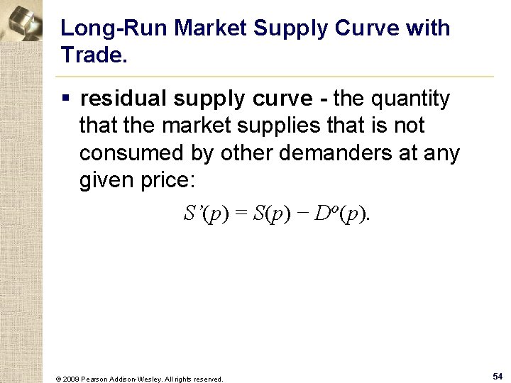
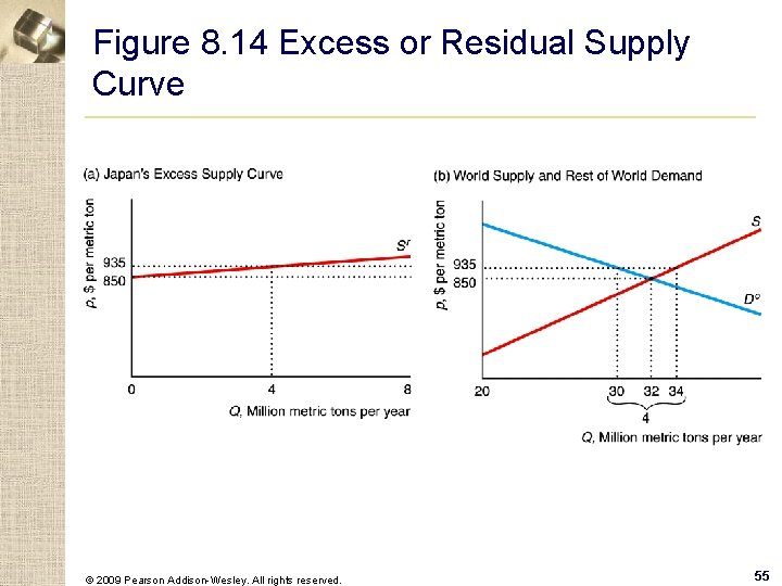
Long-Run Market Supply Curve with Trade. § residual supply curve - the quantity that the market supplies that is not consumed by other demanders at any given price: S’(p) = S(p) − Do(p). © 2009 Pearson Addison-Wesley. All rights reserved. 54

Figure 8. 14 Excess or Residual Supply Curve © 2009 Pearson Addison-Wesley. All rights reserved. 55

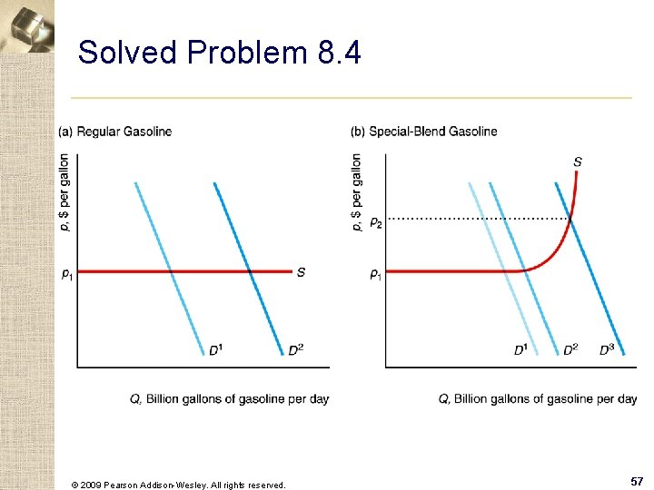
Solved Problem 8. 4 § In the short run, what happens to the competitive market price of gasoline if the demand curve in a state shifts to the right as more people move to the state or start driving gashogging SUVs? In your answer, distinguish between areas in which regular gasoline is sold and jurisdictions that require special blends. © 2009 Pearson Addison-Wesley. All rights reserved. 56

Solved Problem 8. 4 © 2009 Pearson Addison-Wesley. All rights reserved. 57

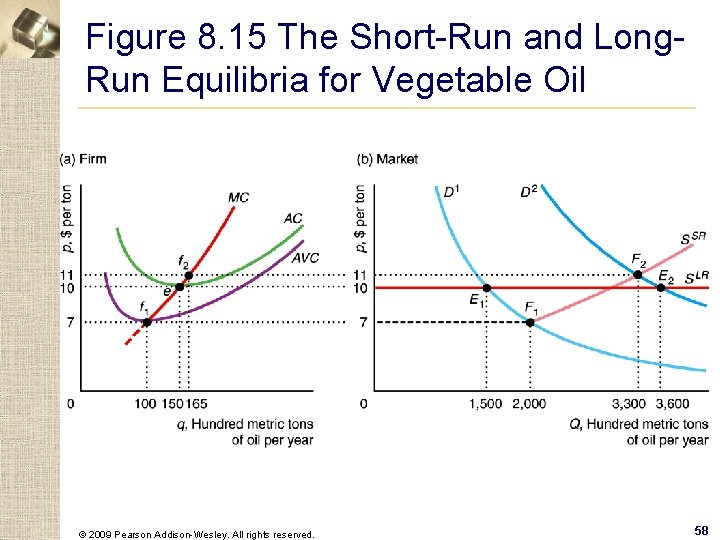
Figure 8. 15 The Short-Run and Long. Run Equilibria for Vegetable Oil © 2009 Pearson Addison-Wesley. All rights reserved. 58

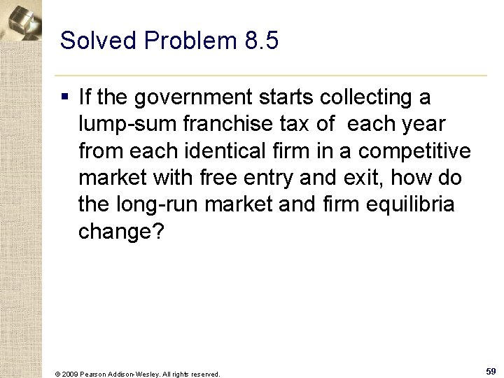
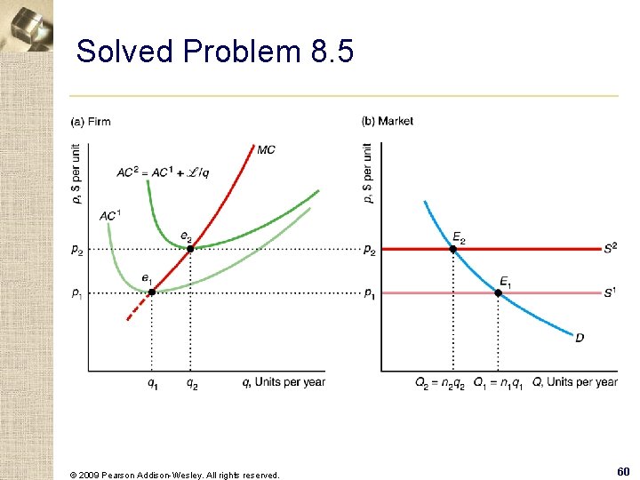
Solved Problem 8. 5 § If the government starts collecting a lump-sum franchise tax of each year from each identical firm in a competitive market with free entry and exit, how do the long-run market and firm equilibria change? © 2009 Pearson Addison-Wesley. All rights reserved. 59

Solved Problem 8. 5 © 2009 Pearson Addison-Wesley. All rights reserved. 60

Zero Long-Run Profit with Free Entry § One implication of the shutdown rule is that the firm is willing to operate in the long run even if it is making zero profit. w But how can this be? w Because opportunity cost includes the value of the next best investment, at a zero longrun economic profit, the firm is earning the normal business profit that the firm could earn by investing elsewhere in the economy. © 2009 Pearson Addison-Wesley. All rights reserved. 61

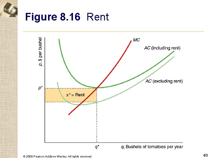
Zero Long-Run Profit When Entry Is Limited § Rent - a payment to the owner of an input beyond the minimum necessary for the factor to be supplied © 2009 Pearson Addison-Wesley. All rights reserved. 62

Figure 8. 16 Rent © 2009 Pearson Addison-Wesley. All rights reserved. 63