Chapter 9 Supervised Learning Neural Networks Introduction 9

Chapter 9: Supervised Learning Neural Networks • Introduction (9. 1) • Perceptrons (9. 2) • Adaline (9. 3) • Backpropagation Multilayer Perceptrons (9. 4) • Radial Basis Function Networks (9. 5) Jyh-Shing Roger Jang et al. , Neuro-Fuzzy and Soft Computing: A Computational Approach to Learning and Machine Intelligence , First Edition, Prentice Hall, 1997

2 Introduction (9. 1) • Artificial Neural Networks (NN) have been studied since 1950 • Minsky & Papert in their report of perceptron (Rosenblatt) expressed pessimism over multilayer systems, the interest in NN dwindled in the 1970’s • The work of Rumelhart, Hinton, Williams & others, in learning algorithms created a resurgence of the lost interest in the field of NN Dr. Djamel Bouchaffra CSE 513 Soft Computing, Ch. 9: Supervised learning Neural Networks

3 Introduction (9. 1) (cont. ) • Several NN have been proposed & investigated in recent years – – Supervised versus unsupervised Architectures (feedforward vs. recurrent) Implementation (software vs. hardware) Operations (biologically inspired vs. psychologically inspired) • In this chapter, we will focus on modeling problems with desired input-output data set, so the resulting networks must have adjustable parameters that are updated by a supervised learning rule Dr. Djamel Bouchaffra CSE 513 Soft Computing, Ch. 9: Supervised learning Neural Networks

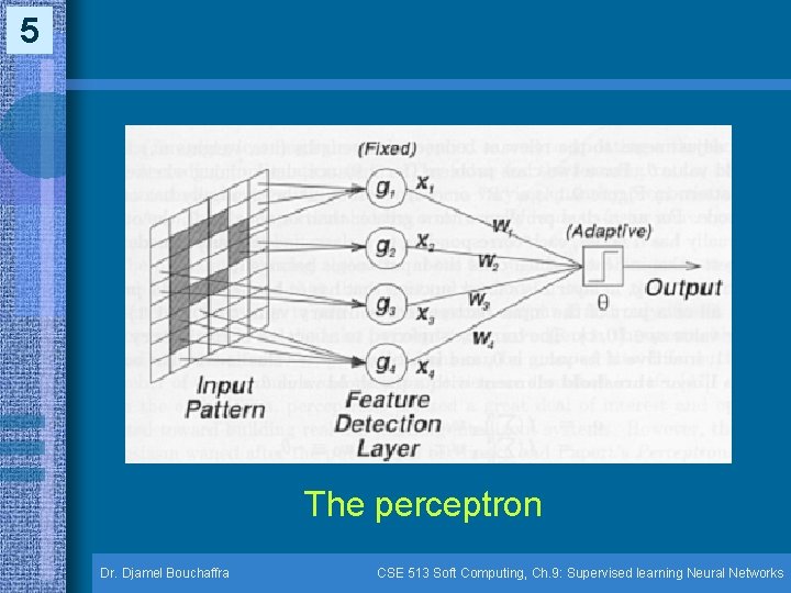
4 Perceptrons (9. 2) • Architecture & learning rule – The perceptron was derived from a biological brain neuron model introduced by Mc Culloch & Pitts in 1943 – Rosenblatt designed the perceptron with a view toward explaining & modeling pattern recognition abilities of biological visual systems – The following figure illustrate a two-class problem that consists of determining whether the input pattern is a “p” or not Dr. Djamel Bouchaffra CSE 513 Soft Computing, Ch. 9: Supervised learning Neural Networks

5 The perceptron Dr. Djamel Bouchaffra CSE 513 Soft Computing, Ch. 9: Supervised learning Neural Networks

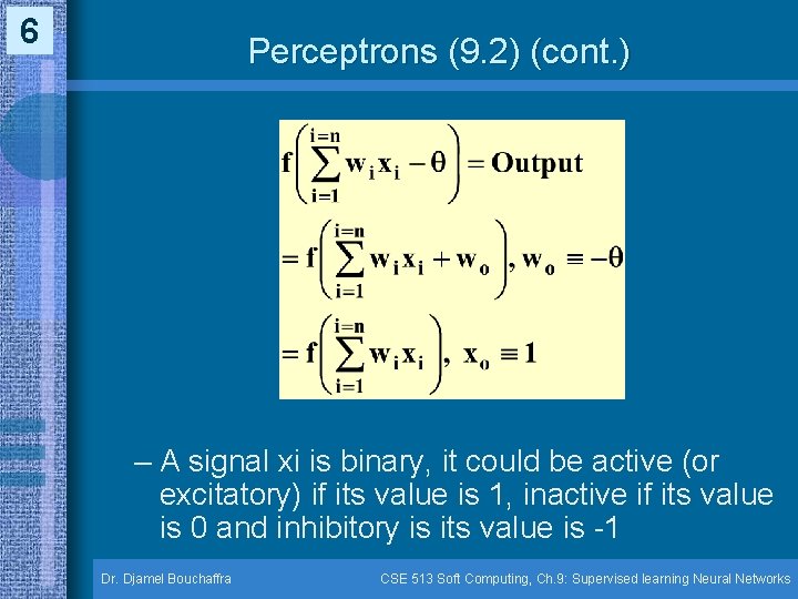
6 Perceptrons (9. 2) (cont. ) – A signal xi is binary, it could be active (or excitatory) if its value is 1, inactive if its value is 0 and inhibitory is its value is -1 Dr. Djamel Bouchaffra CSE 513 Soft Computing, Ch. 9: Supervised learning Neural Networks

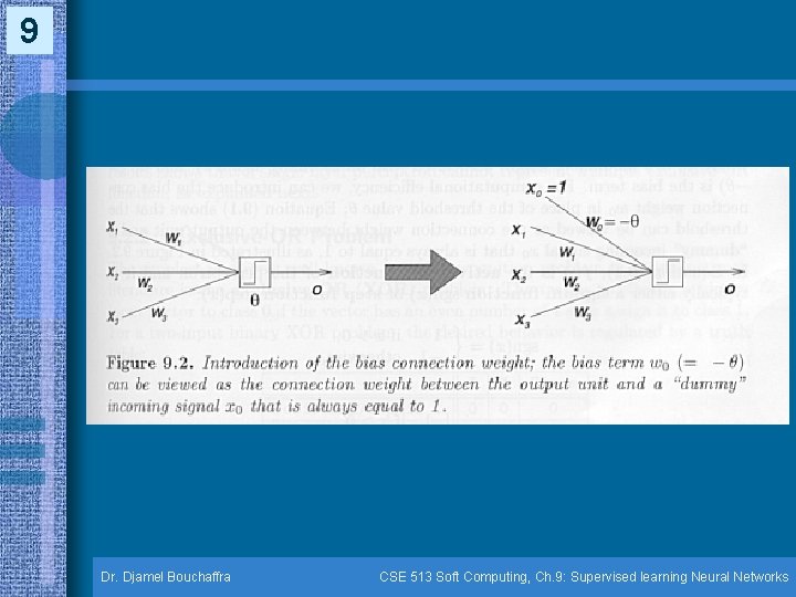
7 Perceptrons (9. 2) (cont. ) • Architecture & learning rule (cont. ) – The output unit is a linear threshold element with a threshold value – wi is a modifiable weight associated with an incoming signal xi – The threshold = w 0 can be viewed as the connection weight between the output unit & a dummy incoming signal x 0 = 1 Dr. Djamel Bouchaffra CSE 513 Soft Computing, Ch. 9: Supervised learning Neural Networks

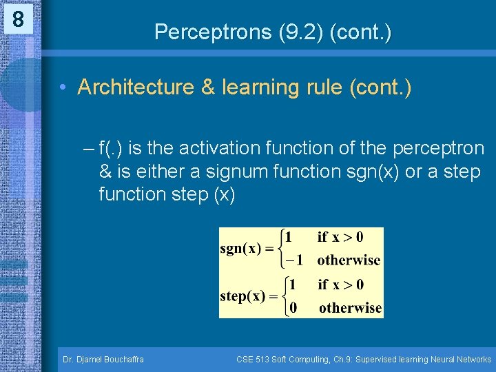
8 Perceptrons (9. 2) (cont. ) • Architecture & learning rule (cont. ) – f(. ) is the activation function of the perceptron & is either a signum function sgn(x) or a step function step (x) Dr. Djamel Bouchaffra CSE 513 Soft Computing, Ch. 9: Supervised learning Neural Networks

9 Dr. Djamel Bouchaffra CSE 513 Soft Computing, Ch. 9: Supervised learning Neural Networks

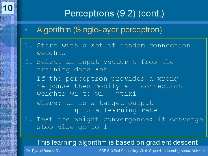
10 Perceptrons (9. 2) (cont. ) • Algorithm (Single-layer perceptron) 1. Start with a set of random connection weights 2. Select an input vector x from the training data set If the perceptron provides a wrong response then modify all connection weights wi to wi = tixi where: ti is a target output is a learning rate 1. Test the weight convergence: if converge stop else go to 1 This learning algorithm is based on gradient descent Dr. Djamel Bouchaffra CSE 513 Soft Computing, Ch. 9: Supervised learning Neural Networks

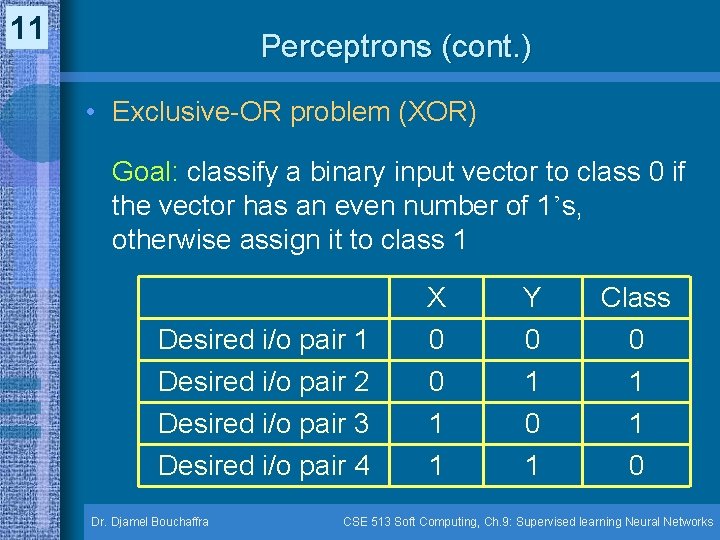
11 Perceptrons (cont. ) • Exclusive-OR problem (XOR) Goal: classify a binary input vector to class 0 if the vector has an even number of 1’s, otherwise assign it to class 1 Desired i/o pair 2 X 0 0 Y 0 1 Class 0 1 Desired i/o pair 3 Desired i/o pair 4 1 1 0 Dr. Djamel Bouchaffra CSE 513 Soft Computing, Ch. 9: Supervised learning Neural Networks

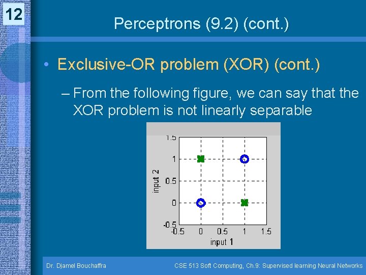
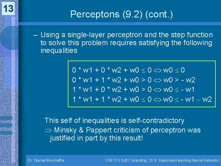
12 Perceptrons (9. 2) (cont. ) • Exclusive-OR problem (XOR) (cont. ) – From the following figure, we can say that the XOR problem is not linearly separable Dr. Djamel Bouchaffra CSE 513 Soft Computing, Ch. 9: Supervised learning Neural Networks

13 Perceptons (9. 2) (cont. ) – Using a single-layer perceptron and the step function to solve this problem requires satisfying the following inequalities 0 * w 1 + 0 * w 2 + w 0 0 0 * w 1 + 1 * w 2 + w 0 > 0 w 0 > - w 2 1 * w 1 + 0 * w 2 + w 0 > 0 w 0 - w 1 1 * w 1 + 1 * w 2 + w 0 0 w 0 - w 1 – w 2 This self of inequalities is self-contradictory Minsky & Pappert criticism of perceptron was justified in part by this result! Dr. Djamel Bouchaffra CSE 513 Soft Computing, Ch. 9: Supervised learning Neural Networks

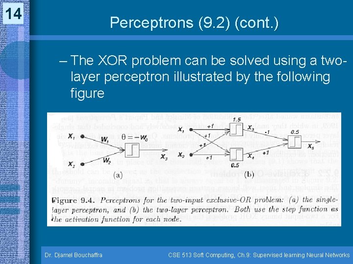
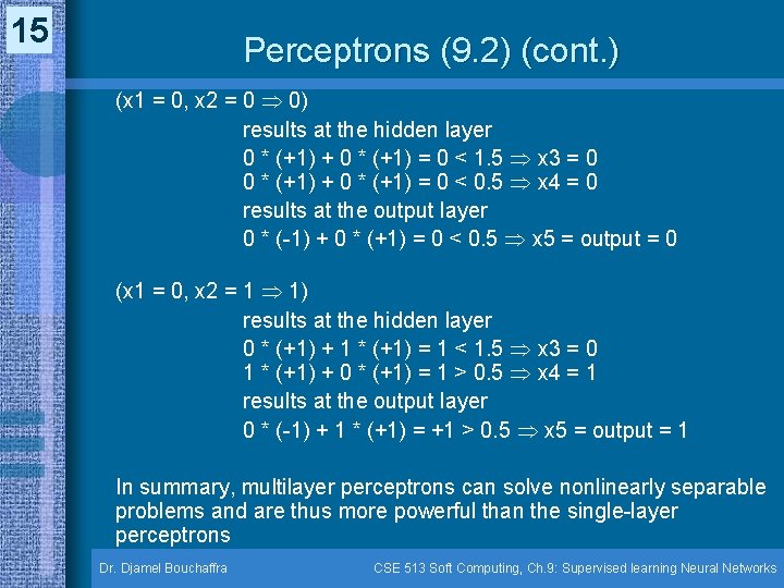
14 Perceptrons (9. 2) (cont. ) – The XOR problem can be solved using a twolayer perceptron illustrated by the following figure Dr. Djamel Bouchaffra CSE 513 Soft Computing, Ch. 9: Supervised learning Neural Networks

15 Perceptrons (9. 2) (cont. ) (x 1 = 0, x 2 = 0 0) results at the hidden layer 0 * (+1) + 0 * (+1) = 0 < 1. 5 x 3 = 0 0 * (+1) + 0 * (+1) = 0 < 0. 5 x 4 = 0 results at the output layer 0 * (-1) + 0 * (+1) = 0 < 0. 5 x 5 = output = 0 (x 1 = 0, x 2 = 1 1) results at the hidden layer 0 * (+1) + 1 * (+1) = 1 < 1. 5 x 3 = 0 1 * (+1) + 0 * (+1) = 1 > 0. 5 x 4 = 1 results at the output layer 0 * (-1) + 1 * (+1) = +1 > 0. 5 x 5 = output = 1 In summary, multilayer perceptrons can solve nonlinearly separable problems and are thus more powerful than the single-layer perceptrons Dr. Djamel Bouchaffra CSE 513 Soft Computing, Ch. 9: Supervised learning Neural Networks

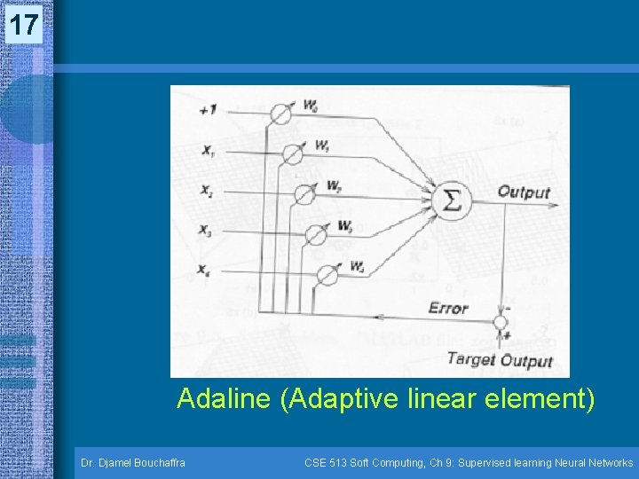
16 ADALINE (9. 3) • Developed by Widrow & Hoff, this model represents a classical example of the simplest intelligent self-learning system that can adapt itself to achieve a given modeling task Dr. Djamel Bouchaffra CSE 513 Soft Computing, Ch. 9: Supervised learning Neural Networks

17 Adaline (Adaptive linear element) Dr. Djamel Bouchaffra CSE 513 Soft Computing, Ch. 9: Supervised learning Neural Networks

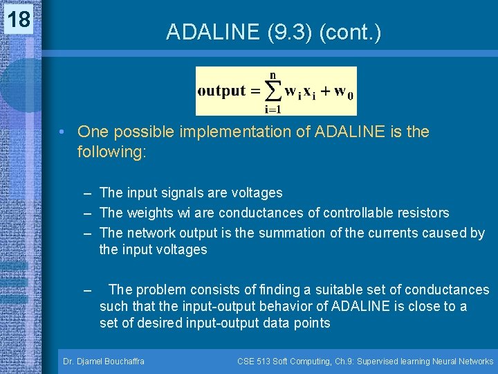
18 ADALINE (9. 3) (cont. ) • One possible implementation of ADALINE is the following: – The input signals are voltages – The weights wi are conductances of controllable resistors – The network output is the summation of the currents caused by the input voltages – The problem consists of finding a suitable set of conductances such that the input-output behavior of ADALINE is close to a set of desired input-output data points Dr. Djamel Bouchaffra CSE 513 Soft Computing, Ch. 9: Supervised learning Neural Networks

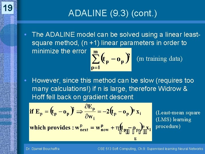
19 ADALINE (9. 3) (cont. ) • The ADALINE model can be solved using a linear leastsquare method, (n +1) linear parameters in order to minimize the error (m training data) • However, since this method can be slow (requires too many calculations!) if n is large, therefore Widrow & Hoff fell back on gradient descent (Least-mean square (LMS) learning procedure) Dr. Djamel Bouchaffra CSE 513 Soft Computing, Ch. 9: Supervised learning Neural Networks

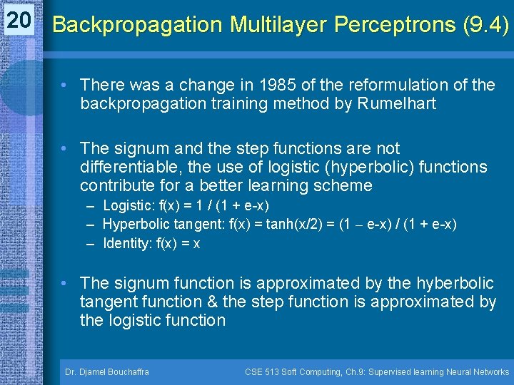
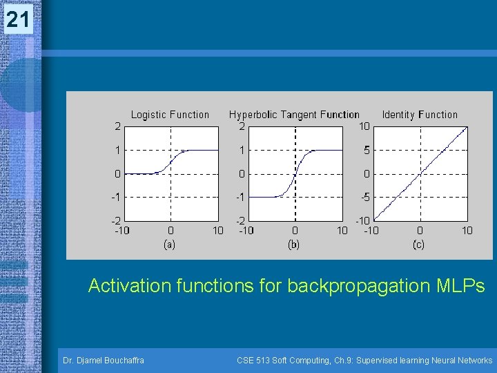
20 Backpropagation Multilayer Perceptrons (9. 4) • There was a change in 1985 of the reformulation of the backpropagation training method by Rumelhart • The signum and the step functions are not differentiable, the use of logistic (hyperbolic) functions contribute for a better learning scheme – Logistic: f(x) = 1 / (1 + e-x) – Hyperbolic tangent: f(x) = tanh(x/2) = (1 – e-x) / (1 + e-x) – Identity: f(x) = x • The signum function is approximated by the hyberbolic tangent function & the step function is approximated by the logistic function Dr. Djamel Bouchaffra CSE 513 Soft Computing, Ch. 9: Supervised learning Neural Networks

21 Activation functions for backpropagation MLPs Dr. Djamel Bouchaffra CSE 513 Soft Computing, Ch. 9: Supervised learning Neural Networks

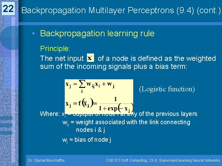
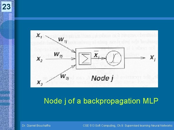
22 Backpropagation Multilayer Perceptrons (9. 4) (cont. ) • Backpropagation learning rule Principle: The net input of a node is defined as the weighted sum of the incoming signals plus a bias term: (Logistic function) Where: xi = ouptput of node i at any of the previous layers wij = weight associated with the link connecting nodes i & j wj = bias of node j Dr. Djamel Bouchaffra CSE 513 Soft Computing, Ch. 9: Supervised learning Neural Networks

23 Node j of a backpropagation MLP Dr. Djamel Bouchaffra CSE 513 Soft Computing, Ch. 9: Supervised learning Neural Networks

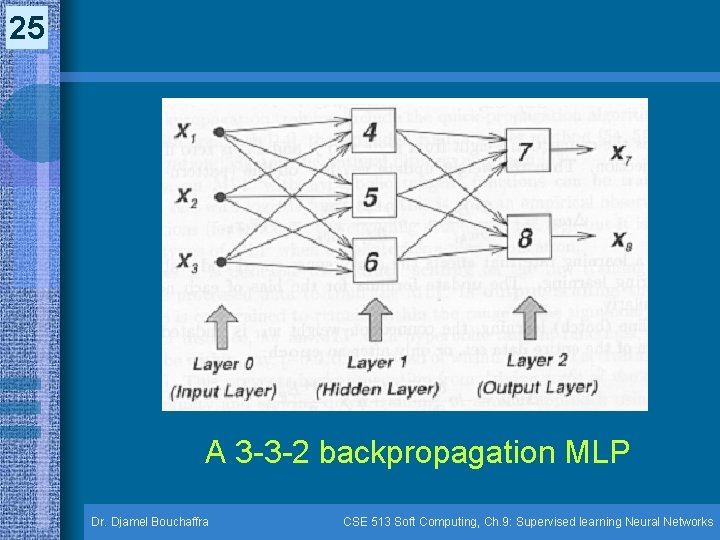
24 Backpropagation Multilayer Perceptrons (9. 4) (cont. ) • The following figure shows a two-layer backpropagation MLP with 3 inputs in the input layer, 3 neurons in the hidden layer & 2 output neurons in the output layer Dr. Djamel Bouchaffra CSE 513 Soft Computing, Ch. 9: Supervised learning Neural Networks

25 A 3 -3 -2 backpropagation MLP Dr. Djamel Bouchaffra CSE 513 Soft Computing, Ch. 9: Supervised learning Neural Networks

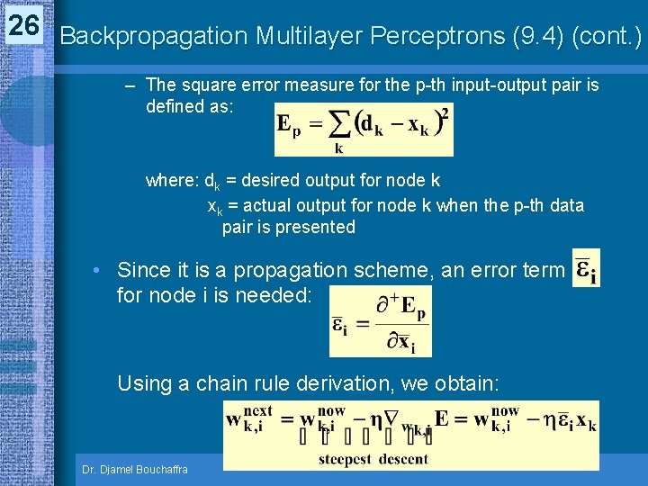
26 Backpropagation Multilayer Perceptrons (9. 4) (cont. ) – The square error measure for the p-th input-output pair is defined as: where: dk = desired output for node k xk = actual output for node k when the p-th data pair is presented • Since it is a propagation scheme, an error term for node i is needed: Using a chain rule derivation, we obtain: Dr. Djamel Bouchaffra

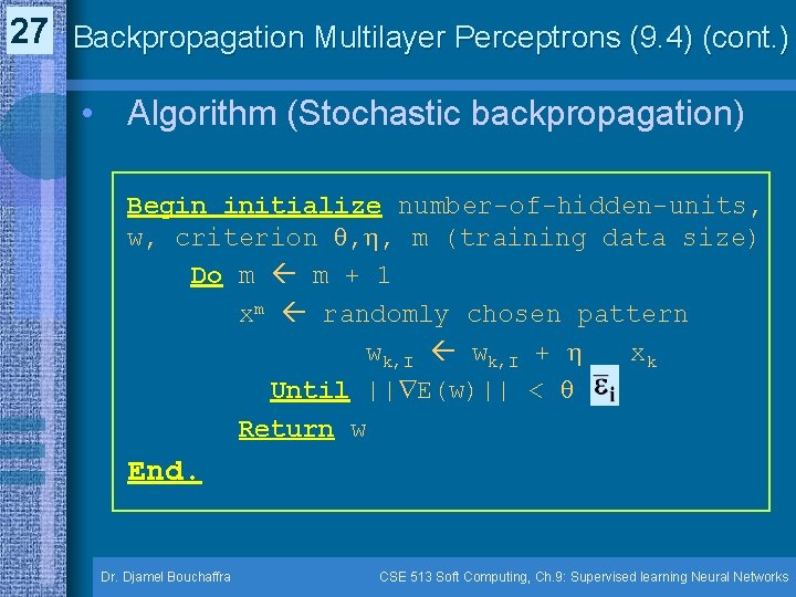
27 Backpropagation Multilayer Perceptrons (9. 4) (cont. ) • Algorithm (Stochastic backpropagation) Begin initialize number-of-hidden-units, w, criterion , , m (training data size) Do m m + 1 xm randomly chosen pattern wk, I + xk Until || E(w)|| < Return w End. Dr. Djamel Bouchaffra CSE 513 Soft Computing, Ch. 9: Supervised learning Neural Networks

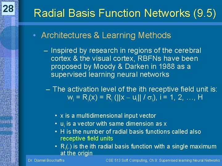
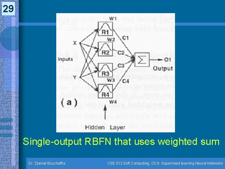
28 Radial Basis Function Networks (9. 5) • Architectures & Learning Methods – Inspired by research in regions of the cerebral cortex & the visual cortex, RBFNs have been proposed by Moody & Darken in 1988 as a supervised learning neural networks – The activation level of the ith receptive field unit is: wi = Ri(x) = Ri (||x – ui|| / i), i = 1, 2, …, H • x is a multidimensional input vector • ui is a vector with same dimension as x • H is the number of radial basis functions called also receptive field units • Ri(. ) is the ith radial basis function with a single maximum at the origin Dr. Djamel Bouchaffra CSE 513 Soft Computing, Ch. 9: Supervised learning Neural Networks

29 Single-output RBFN that uses weighted sum Dr. Djamel Bouchaffra CSE 513 Soft Computing, Ch. 9: Supervised learning Neural Networks

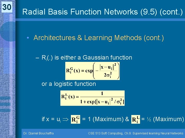
30 Radial Basis Function Networks (9. 5) (cont. ) • Architectures & Learning Methods (cont. ) – Ri(. ) is either a Gaussian function or a logistic function if x = ui Dr. Djamel Bouchaffra = 1 (Maximum) & = ½ (Maximum) CSE 513 Soft Computing, Ch. 9: Supervised learning Neural Networks

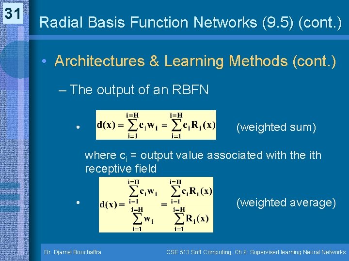
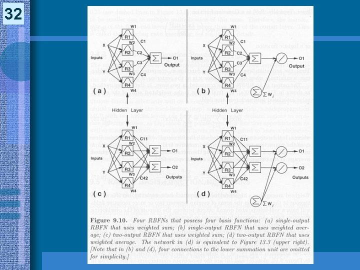
31 Radial Basis Function Networks (9. 5) (cont. ) • Architectures & Learning Methods (cont. ) – The output of an RBFN • (weighted sum) where ci = output value associated with the ith receptive field • Dr. Djamel Bouchaffra (weighted average) CSE 513 Soft Computing, Ch. 9: Supervised learning Neural Networks

32

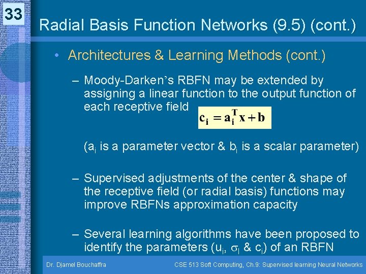
33 Radial Basis Function Networks (9. 5) (cont. ) • Architectures & Learning Methods (cont. ) – Moody-Darken’s RBFN may be extended by assigning a linear function to the output function of each receptive field (ai is a parameter vector & bi is a scalar parameter) – Supervised adjustments of the center & shape of the receptive field (or radial basis) functions may improve RBFNs approximation capacity – Several learning algorithms have been proposed to identify the parameters (ui, I & ci) of an RBFN Dr. Djamel Bouchaffra CSE 513 Soft Computing, Ch. 9: Supervised learning Neural Networks

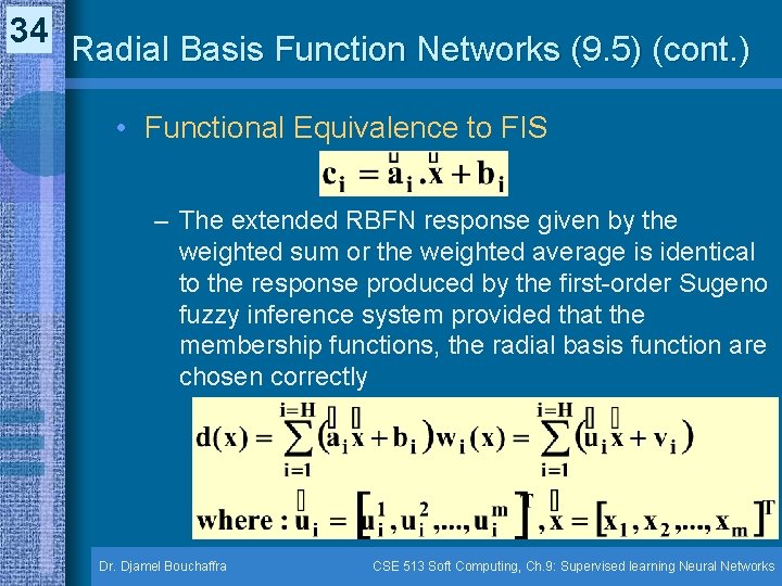
34 Radial Basis Function Networks (9. 5) (cont. ) • Functional Equivalence to FIS – The extended RBFN response given by the weighted sum or the weighted average is identical to the response produced by the first-order Sugeno fuzzy inference system provided that the membership functions, the radial basis function are chosen correctly Dr. Djamel Bouchaffra CSE 513 Soft Computing, Ch. 9: Supervised learning Neural Networks

35 Radial Basis Function Networks (9. 5) (cont. ) • Functional Equivalence to FIS (CONT. ) – While the RBFN consists of radial basis functions, the FIS comprises a certain number of membership functions – The FIS & the RBFN were developed on different bases, they are rooted in the same soil Dr. Djamel Bouchaffra CSE 513 Soft Computing, Ch. 9: Supervised learning Neural Networks

36 Radial Basis Function Networks (9. 5)(cont. ) • Functional Equivalence to FIS (cont. ) – Condition of equivalence between FIS & RBFN • RBFN & FIS use both of them the same aggregation method (weighted average & weighted sum) • The number of receptive field units in RBFN is equal to the number of fuzzy if-then rules in the FIS • Each radial basis function of the RBFN is equal to a multidimensional composite MF of the premise part of a fuzzy rule in the FIS • Corresponding radial basis & fuzzy rule should have the same response function Dr. Djamel Bouchaffra CSE 513 Soft Computing, Ch. 9: Supervised learning Neural Networks

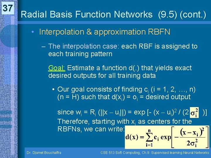
37 Radial Basis Function Networks (9. 5) (cont. ) • Interpolation & approximation RBFN – The interpolation case: each RBF is assigned to each training pattern Goal: Estimate a function d(. ) that yields exact desired outputs for all training data • Our goal consists of finding ci (i = 1, 2, …, n) (n = H) such that d(xi) = oi = desired output since wi = Ri (||x – ui||) = exp [- (x – ui)2 / (2 Therefore, starting with xi as centers for the RBFNs, we can write: Dr. Djamel Bouchaffra )] CSE 513 Soft Computing, Ch. 9: Supervised learning Neural Networks

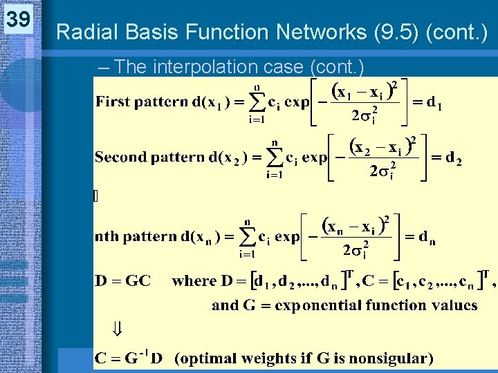
38 Radial Basis Function Networks (9. 5) (cont. ) • Interpolation & approximation RBFN (cont. ) – The interpolation case (cont. ) • For given i (i = 1, …, n), we obtain the following n simultaneous linear equations with respect to unknown weights ci (i = 1, 2, …, n)

39 Radial Basis Function Networks (9. 5) (cont. ) – The interpolation case (cont. )

40 Radial Basis Function Networks (9. 5) (cont. ) • Interpolation & approximation RBFN (cont. ) – Approximation RBFN • This corresponds to the case when there are fewer basis functions than there available training patterns • In this case, the matrix G is rectangular & the least square methods are commonly used in order to find the vector C Dr. Djamel Bouchaffra CSE 513 Soft Computing, Ch. 9: Supervised learning Neural Networks