CHAPTER 9 Statistical Physics n underpins thermodynamics ideal

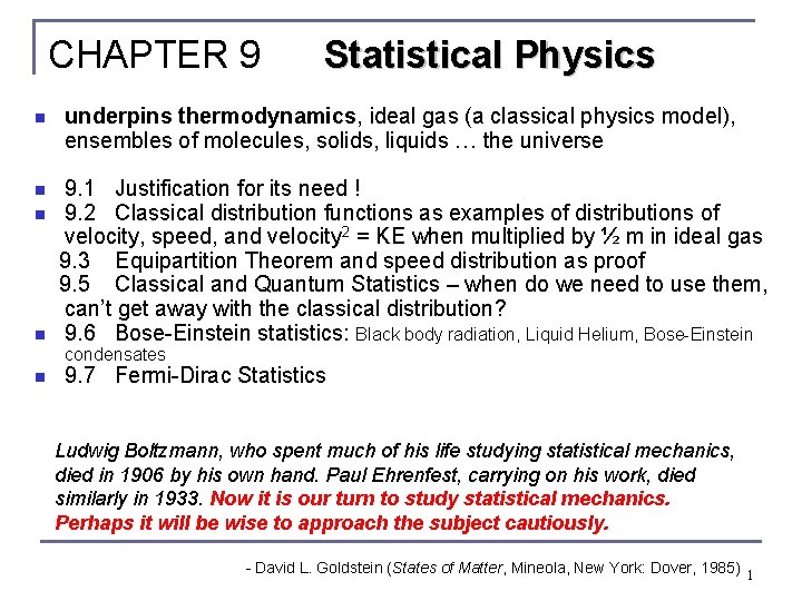
CHAPTER 9 Statistical Physics n underpins thermodynamics, ideal gas (a classical physics model), ensembles of molecules, solids, liquids … the universe 9. 1 Justification for its need ! n 9. 2 Classical distribution functions as examples of distributions of velocity, speed, and velocity 2 = KE when multiplied by ½ m in ideal gas 9. 3 Equipartition Theorem and speed distribution as proof 9. 5 Classical and Quantum Statistics – when do we need to use them, can’t get away with the classical distribution? n 9. 6 Bose-Einstein statistics: Black body radiation, Liquid Helium, Bose-Einstein n condensates n 9. 7 Fermi-Dirac Statistics Ludwig Boltzmann, who spent much of his life studying statistical mechanics, died in 1906 by his own hand. Paul Ehrenfest, carrying on his work, died similarly in 1933. Now it is our turn to study statistical mechanics. Perhaps it will be wise to approach the subject cautiously. - David L. Goldstein (States of Matter, Mineola, New York: Dover, 1985) 1

First there was classical physics with a cause (or causes) Newton’s three force laws, first unification in physics Lagrange around 1790 and Hamilton around 1840 added significantly to the computational power of Newtonian mechanics. Pierre-Simon de Laplace (1749 -1827) made major contributions to theory of probability and the well-known clockwork universe statement: It should be possible in principle to have perfect knowledge of the universe. Such knowledge would come from measuring at one time the position and velocities of every particle of matter and then applying Newton’s law. As they are cause and effect relations that work forwards and backwards in time, perfect knowledge can be extended all the way back to the beginning of the universe and all the way forward to its end. So no uncertainty principle allowed … 2

then there was the realization that one does not always need to know the cause (causes), can do statistical analyses instead Typical problem, flipping of 100 coins, One can try to identify all physical condition before the toss, model the toss itself, and then predict how the coin will fall down if all done correctly, one will be able to make a prediction on how many heads or tails one will obtain in a series of experiments Statistics and probabilities would just predict 50 % heads 50% tails by ignoring all of that physics, The more experimental trials, 100, 000 coin tosses, the better this prediction will be borne out The field of statistical (macroscopic) physics that is concerned with the effects of many particle at once 3

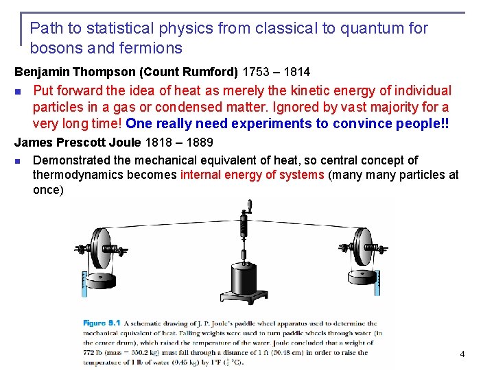
Path to statistical physics from classical to quantum for bosons and fermions Benjamin Thompson (Count Rumford) 1753 – 1814 n Put forward the idea of heat as merely the kinetic energy of individual particles in a gas or condensed matter. Ignored by vast majority for a very long time! One really need experiments to convince people!! James Prescott Joule 1818 – 1889 n Demonstrated the mechanical equivalent of heat, so central concept of thermodynamics becomes internal energy of systems (many particles at once) 4

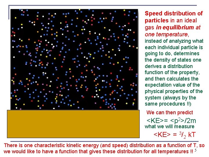
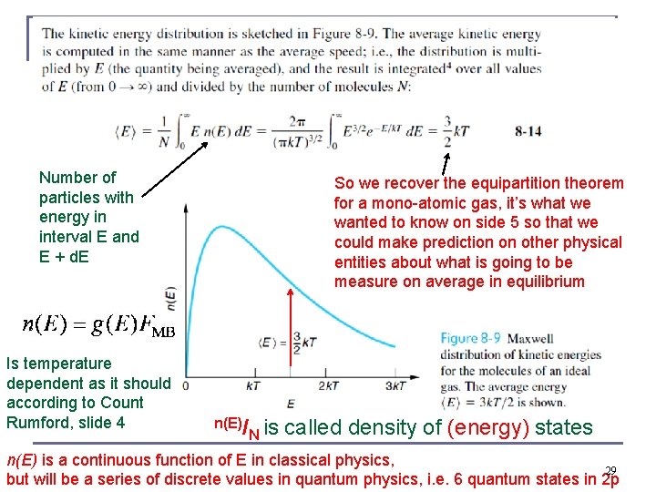
Speed distribution of particles in an ideal gas in equilibrium at one temperature, instead of analyzing what each individual particle is going to do, determines the density of states one derives a distribution function of the property, and then calculates the expectation value of the physical properties of the system (always by the same procedures !!) We can then predict <KE>= <p 2>/2 m what we will measure <KE> = 3/2 k. T There is one characteristic kinetic energy (and speed) distribution as a function of T, so we would like to have a function that gives these distribution for all temperatures !! 5

Beyond first and second year college physics James Clark Maxwell 1831 – 1879, Josiah Willard Gibbs 1839 – 1903, Ludwig Boltzmann 1844 – 1906 (all believed in reality of atoms, tiny minority at that time) Brought the mathematical theories of probability and observational statistics to bear on the physical thermodynamics problems of their time. Showed that statistical distributions of physical properties of an ideal gas (in equilibrium – a stationary state) can be used to explain the observed classical macroscopic phenomena (i. e. well-known gas laws) Gibbs invents notation for vector calculus, the form in which we use Maxwell’s equations today Maxwell’s electromagnetic theory succeeded his work on statistical foundation of thermodynamics – so he was a genius twice over. 6

and then there came modern physics … Einstein 1905 n Ph. D thesis, the correct theory of Brownian motion, a theory that required atoms to be real, because there are measurable consequences to their motion, (also start of quantitative nanoscience as size of a common sugar molecule (≈ 1 nm) was determined correctly) Bose (with Einstein’s generalization) 1924 n Statistics of indistinguishable particles that are bosons (photons: Bose, all other bosons: Einstein’s generalization) Fermi and Dirac independently 1926 n Statistics of indistinguishable particles that are fermions Procedure is always: we have a part of the distribution function that is property specific (deriving this is the ingenious physics bit) and one of three characteristic statistical expressions for each of the three different types of particles. The product-function of these two factor-functions is the distribution function for the problem at hand. From the distribution function we calculate expectation values, i. e. make predictions. (The relationships between the 7 various physical entities are just the same as in classical/quantum physics)

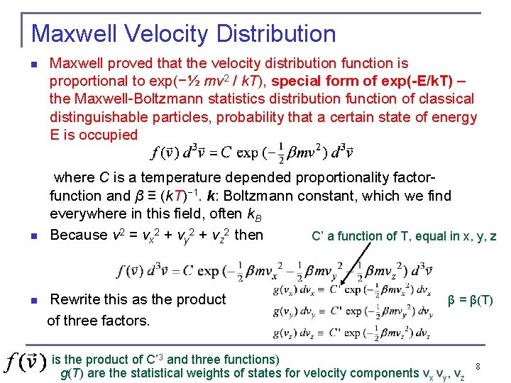
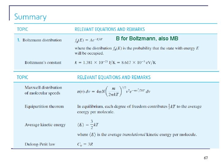
Maxwell Velocity Distribution n n Maxwell proved that the velocity distribution function is proportional to exp(−½ mv 2 / k. T), special form of exp(-E/k. T) – the Maxwell-Boltzmann statistics distribution function of classical distinguishable particles, probability that a certain state of energy E is occupied where C is a temperature depended proportionality factorfunction and β ≡ (k. T)− 1. k: Boltzmann constant, which we find everywhere in this field, often k. B Because v 2 = vx 2 + vy 2 + vz 2 then C’ a function of T, equal in x, y, z Rewrite this as the product of three factors. n β = β(T) is the product of C’ 3 and three functions) g(T) are the statistical weights of states for velocity components vx vy, vz 8

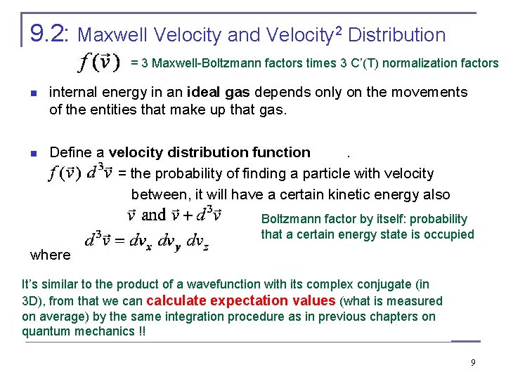
9. 2: Maxwell Velocity and Velocity 2 Distribution = 3 Maxwell-Boltzmann factors times 3 C’(T) normalization factors n internal energy in an ideal gas depends only on the movements of the entities that make up that gas. Define a velocity distribution function. = the probability of finding a particle with velocity between, it will have a certain kinetic energy also . Boltzmann factor by itself: probability that a certain energy state is occupied where n It’s similar to the product of a wavefunction with its complex conjugate (in 3 D), from that we can calculate expectation values (what is measured on average) by the same integration procedure as in previous chapters on quantum mechanics !! 9

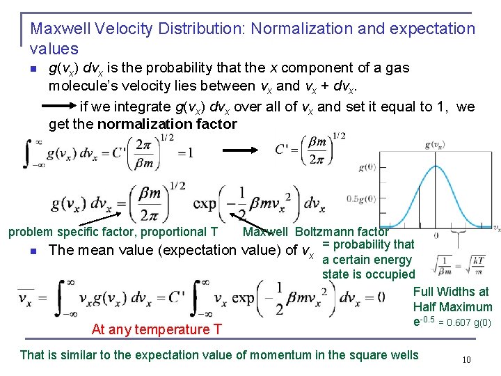
Maxwell Velocity Distribution: Normalization and expectation values n g(vx) dvx is the probability that the x component of a gas molecule’s velocity lies between vx and vx + dvx. if we integrate g(vx) dvx over all of vx and set it equal to 1, we get the normalization factor problem specific factor, proportional T n Maxwell Boltzmann factor The mean value (expectation value) of vx = probability that a certain energy state is occupied Full Widths at Half Maximum e-0. 5 = 0. 607 g(0) At any temperature T That is similar to the expectation value of momentum in the square wells 10

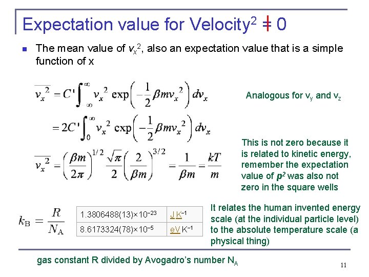
Expectation value for Velocity 2 = 0 n The mean value of vx 2, also an expectation value that is a simple function of x Analogous for vy and vz This is not zero because it is related to kinetic energy, remember the expectation value of p 2 was also not zero in the square wells 1. 3806488(13)× 10− 23 J K− 1 8. 6173324(78)× 10− 5 e. V K− 1 It relates the human invented energy scale (at the individual particle level) to the absolute temperature scale (a physical thing) gas constant R divided by Avogadro’s number NA 11

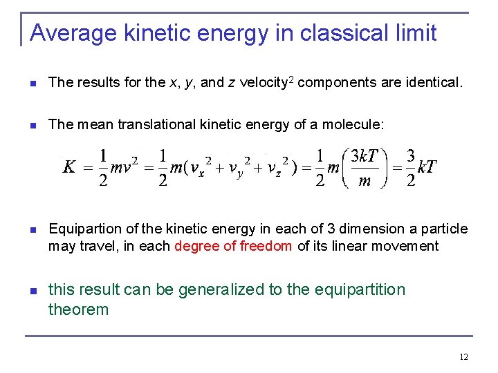
Average kinetic energy in classical limit n The results for the x, y, and z velocity 2 components are identical. n The mean translational kinetic energy of a molecule: n Equipartion of the kinetic energy in each of 3 dimension a particle may travel, in each degree of freedom of its linear movement n this result can be generalized to the equipartition theorem 12

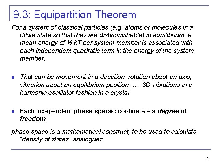
9. 3: Equipartition Theorem For a system of classical particles (e. g. atoms or molecules in a dilute state so that they are distinguishable) in equilibrium, a mean energy of ½ k. T per system member is associated with each independent quadratic term in the energy of the system member. n That can be movement in a direction, rotation about an axis, vibration about an equilibrium position, …, 3 D vibrations in a harmonic oscillator fashion in a crystal n Each independent phase space coordinate = a degree of freedom phase space is a mathematical construct, to be used to calculate “density of states” analogues 13

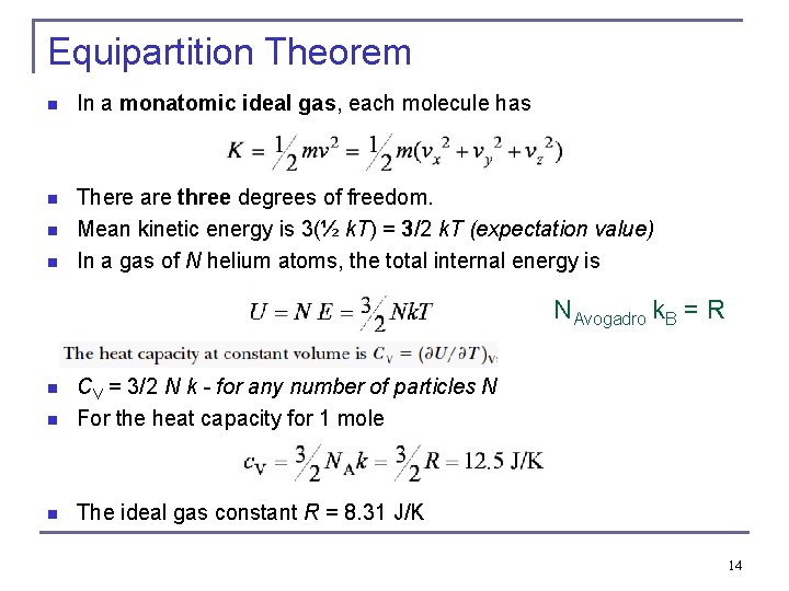
Equipartition Theorem n In a monatomic ideal gas, each molecule has n There are three degrees of freedom. Mean kinetic energy is 3(½ k. T) = 3/2 k. T (expectation value) In a gas of N helium atoms, the total internal energy is n n NAvogadro k. B = R n CV = 3/2 N k - for any number of particles N For the heat capacity for 1 mole n The ideal gas constant R = 8. 31 J/K n 14

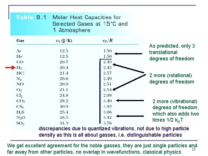
As predicted, only 3 translational degrees of freedom 2 more (rotational) degrees of freedom 2 more (vibrational) degrees of freedom, which also adds two times 1/2 k. BT discrepancies due to quantized vibrations, not due to high particle density as this is all about gasses, i. e. distinguishable particles We get excellent agreement for the noble gasses, they are just single particles and 15 far away from other particles, no overlap in wavefunctions, classical physics

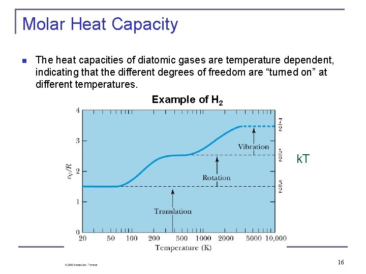
Molar Heat Capacity n The heat capacities of diatomic gases are temperature dependent, indicating that the different degrees of freedom are “turned on” at different temperatures. Example of H 2 k. T 16

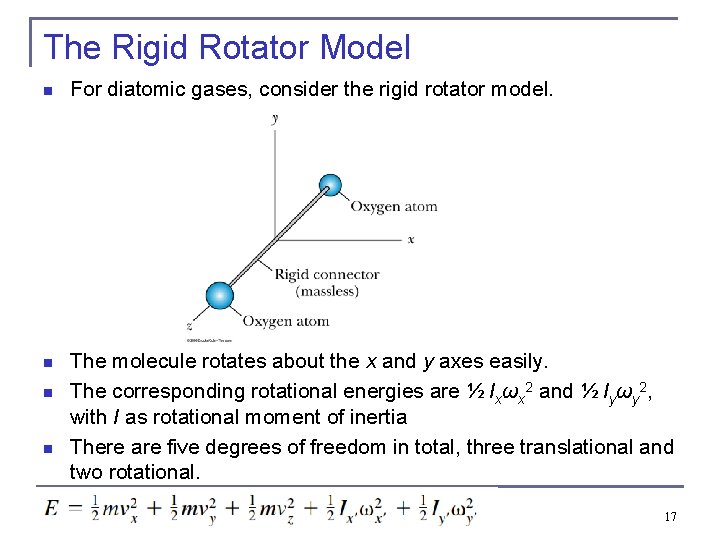
The Rigid Rotator Model n For diatomic gases, consider the rigid rotator model. n The molecule rotates about the x and y axes easily. The corresponding rotational energies are ½ Ixωx 2 and ½ Iyωy 2, with I as rotational moment of inertia There are five degrees of freedom in total, three translational and two rotational. n n 17

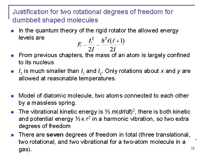
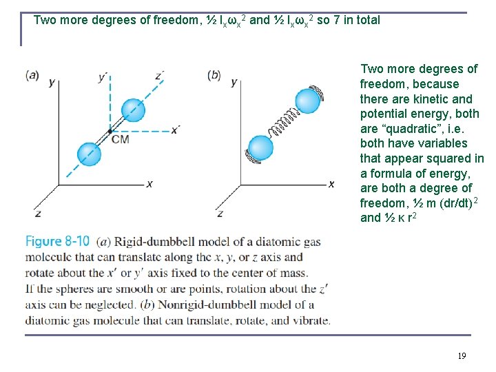
Justification for two rotational degrees of freedom for dumbbell shaped molecules n In the quantum theory of the rigid rotator the allowed energy levels are n From previous chapters, the mass of an atom is largely confined to its nucleus Iz is much smaller than Ix and Iy. Only rotations about x and y are allowed at reasonable temperatures. n n Model of diatomic molecule, two atoms connected to each other by a massless spring. The vibrational kinetic energy is ½ m(dr/dt)2, there is both kinetic and potential energy ½ κ r 2 in a harmonic vibration, so two extra degrees of freedom There are seven degrees of freedom in total (three translational, two rotational, and two vibrational for a two-atom molecule in a 18 gas).

Two more degrees of freedom, ½ Ixωx 2 and ½ Ixωx 2 so 7 in total Two more degrees of freedom, because there are kinetic and potential energy, both are “quadratic”, i. e. both have variables that appear squared in a formula of energy, are both a degree of freedom, ½ m (dr/dt)2 and ½ κ r 2 19

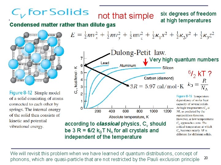
not that simple Condensed matter rather than dilute gas six degrees of freedom at high temperatures Very high quantum numbers 6/ 2 k. T ? according to classical physics, Cv should be 3 R = 6/2 k. BT NA for all crystals and independent of the temperature We will revisit this problem when we have learned of quantum distributions, concept of phonons, which are quasi-particle that are not restricted by the Pauli exclusion principle 20

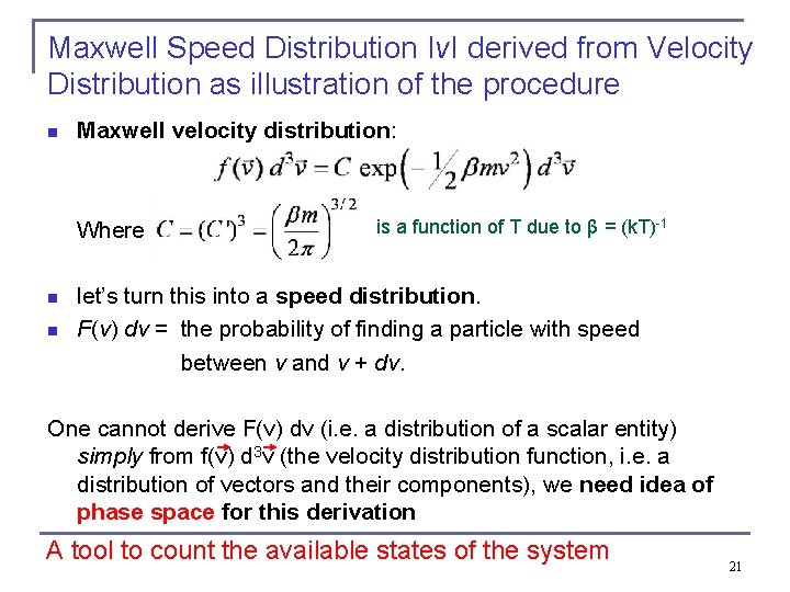
Maxwell Speed Distribution ΙvΙ derived from Velocity Distribution as illustration of the procedure n Maxwell velocity distribution: Where n n is a function of T due to β = (k. T)-1 let’s turn this into a speed distribution. F(v) dv = the probability of finding a particle with speed between v and v + dv. One cannot derive F(v) dv (i. e. a distribution of a scalar entity) simply from f(v) d 3 v (the velocity distribution function, i. e. a distribution of vectors and their components), we need idea of phase space for this derivation A tool to count the available states of the system 21

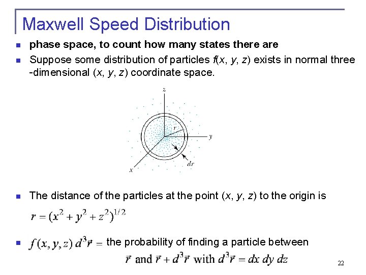
Maxwell Speed Distribution n phase space, to count how many states there are Suppose some distribution of particles f(x, y, z) exists in normal three -dimensional (x, y, z) coordinate space. n The distance of the particles at the point (x, y, z) to the origin is n n the probability of finding a particle between . 22

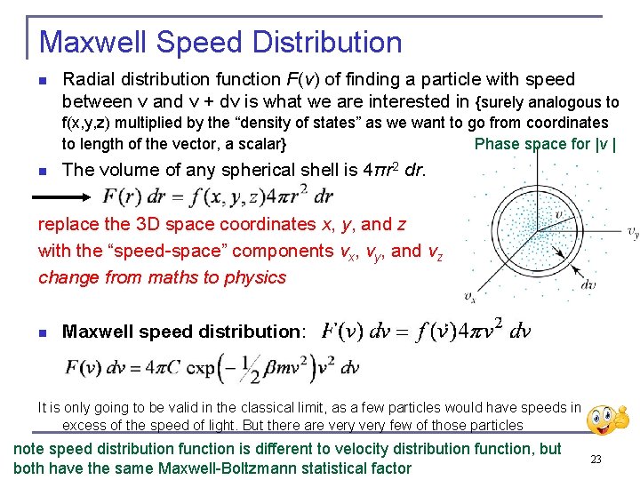
Maxwell Speed Distribution n Radial distribution function F(v) of finding a particle with speed between v and v + dv is what we are interested in {surely analogous to f(x, y, z) multiplied by the “density of states” as we want to go from coordinates Phase space for |v | to length of the vector, a scalar} n The volume of any spherical shell is 4πr 2 dr. replace the 3 D space coordinates x, y, and z with the “speed-space” components vx, vy, and vz change from maths to physics n Maxwell speed distribution: It is only going to be valid in the classical limit, as a few particles would have speeds in excess of the speed of light. But there are very few of those particles note speed distribution function is different to velocity distribution function, but both have the same Maxwell-Boltzmann statistical factor 23

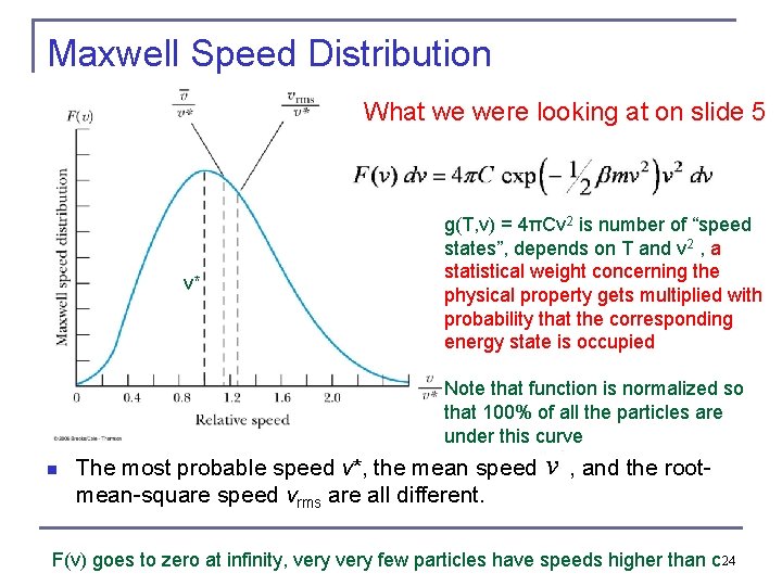
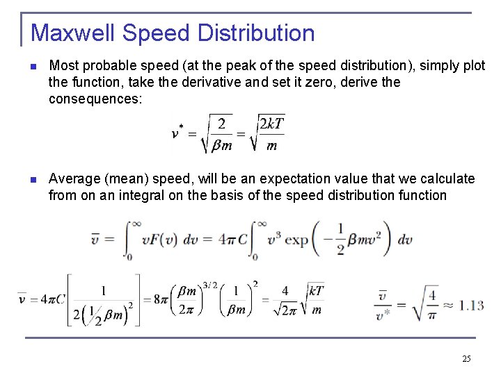
Maxwell Speed Distribution What we were looking at on slide 5 v* g(T, v) = 4πCv 2 is number of “speed states”, depends on T and v 2 , a statistical weight concerning the physical property gets multiplied with probability that the corresponding energy state is occupied Note that function is normalized so that 100% of all the particles are under this curve n The most probable speed v*, the mean speed , and the rootmean-square speed vrms are all different. F(v) goes to zero at infinity, very few particles have speeds higher than c 24

Maxwell Speed Distribution n Most probable speed (at the peak of the speed distribution), simply plot the function, take the derivative and set it zero, derive the consequences: n Average (mean) speed, will be an expectation value that we calculate from on an integral on the basis of the speed distribution function 25

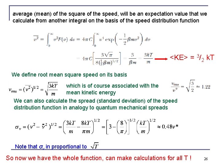
average (mean) of the square of the speed, will be an expectation value that we calculate from another integral on the basis of the speed distribution function <KE> = 3/2 k. T We define root mean square speed on its basis which is of course associated with the mean kinetic energy We can also calculate the spread (standard deviation) of the speed distribution function in analogy to quantum mechanical spreads Note that σv in proportional to So now we have the whole function, can make calculations for all T ! 26

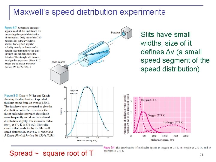
Maxwell’s speed distribution experiments Slits have small widths, size of it defines Δv (a small speed segment of the speed distribution) Spread ~ square root of T 27

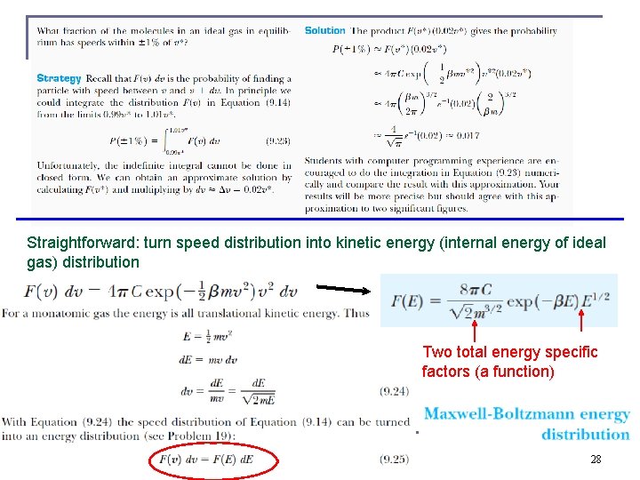
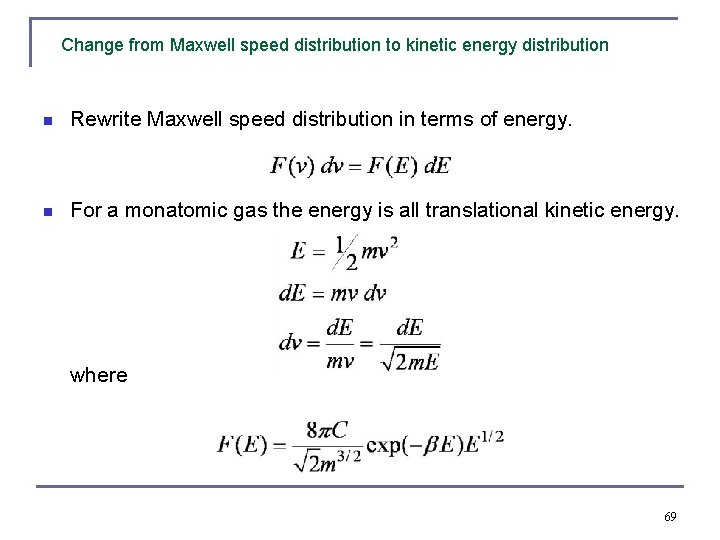
Straightforward: turn speed distribution into kinetic energy (internal energy of ideal gas) distribution Two total energy specific factors (a function) 28

Number of particles with energy in interval E and E + d. E Is temperature dependent as it should according to Count Rumford, slide 4 So we recover the equipartition theorem for a mono-atomic gas, it’s what we wanted to know on side 5 so that we could make prediction on other physical entities about what is going to be measure on average in equilibrium n(E)/ N is called density of (energy) states n(E) is a continuous function of E in classical physics, 29 but will be a series of discrete values in quantum physics, i. e. 6 quantum states in 2 p

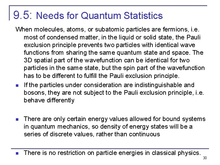
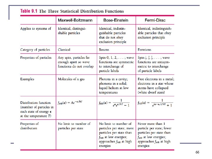
9. 5: Needs for Quantum Statistics When molecules, atoms, or subatomic particles are fermions, i. e. most of condensed matter, in the liquid or solid state, the Pauli exclusion principle prevents two particles with identical wave functions from sharing the same quantum state and space. The 3 D spatial part of the wavefunction can be identical for two particles in the same state, but the spin part of the wavefunction has to be different to fulfill the Pauli exclusion principle. n If the particles under consideration are indistinguishable and bosons, they are not subject to the Pauli exclusion principle, i. e. behave differently n There are only certain energy values allowed for bound systems in quantum mechanics, so density of energy states will be a series of discrete values, rather than continuous n There is no restriction on particle energies in classical physics. 30

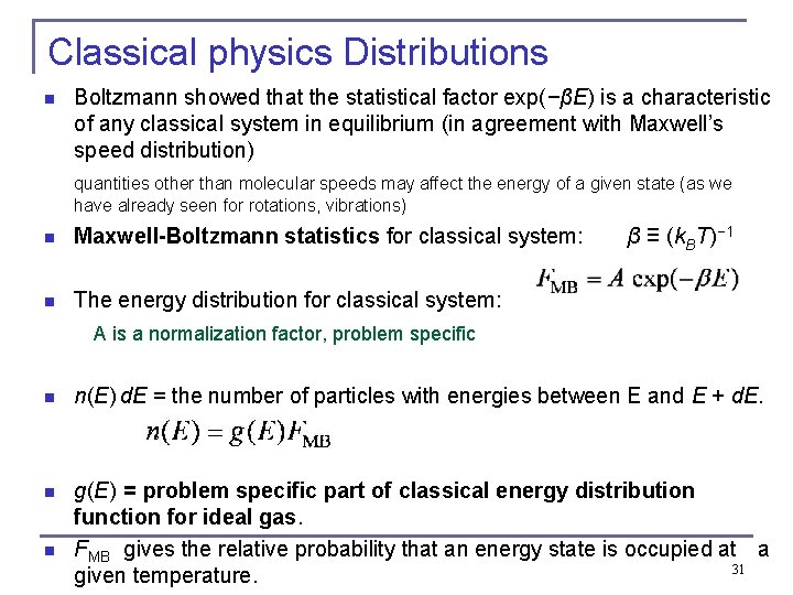
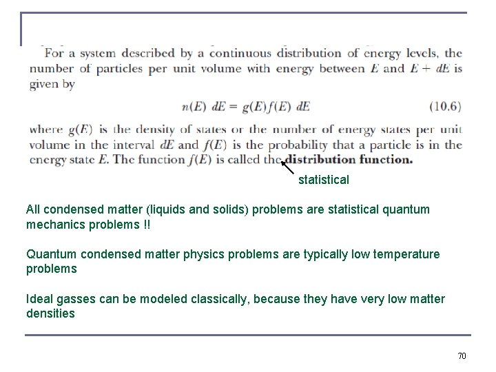
Classical physics Distributions n Boltzmann showed that the statistical factor exp(−βE) is a characteristic of any classical system in equilibrium (in agreement with Maxwell’s speed distribution) quantities other than molecular speeds may affect the energy of a given state (as we have already seen for rotations, vibrations) n Maxwell-Boltzmann statistics for classical system: β ≡ (k. BT)− 1 n The energy distribution for classical system: A is a normalization factor, problem specific n n(E) d. E = the number of particles with energies between E and E + d. E. n g(E) = problem specific part of classical energy distribution function for ideal gas. FMB gives the relative probability that an energy state is occupied at a 31 given temperature. n

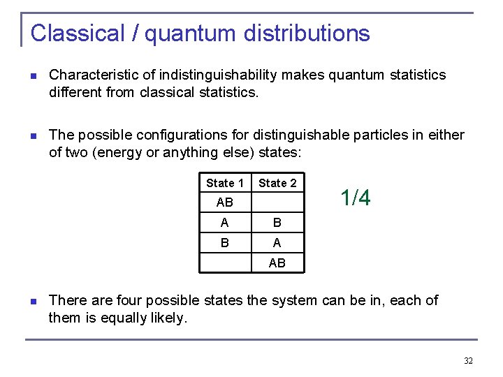
Classical / quantum distributions n Characteristic of indistinguishability makes quantum statistics different from classical statistics. n The possible configurations for distinguishable particles in either of two (energy or anything else) states: State 1 State 2 AB A B B A 1/4 AB n There are four possible states the system can be in, each of them is equally likely. 32

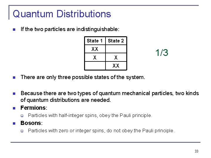
Quantum Distributions n If the two particles are indistinguishable: State 1 State 2 XX X X 1/3 XX n There are only three possible states of the system. n Because there are two types of quantum mechanical particles, two kinds of quantum distributions are needed. Fermions: n q n Particles with half-integer spins, obey the Pauli principle. Bosons: q Particles with zero or integer spins, do not obey the Pauli principle. 33

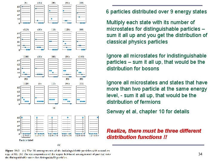
6 particles distributed over 9 energy states Multiply each state with its number of microstates for distinguishable particles – sum it all up and you get the distribution of classical physics particles Ignore all microstates for indistinguishable particles – sum it all up, that would be the distribution for bosons Ignore all microstates and states that have more than two particle at the same energy level, - sum it all up, that would be the distribution of fermions Serway et al, chapter 10 for details Realize, there must be three different distribution functions !! 34

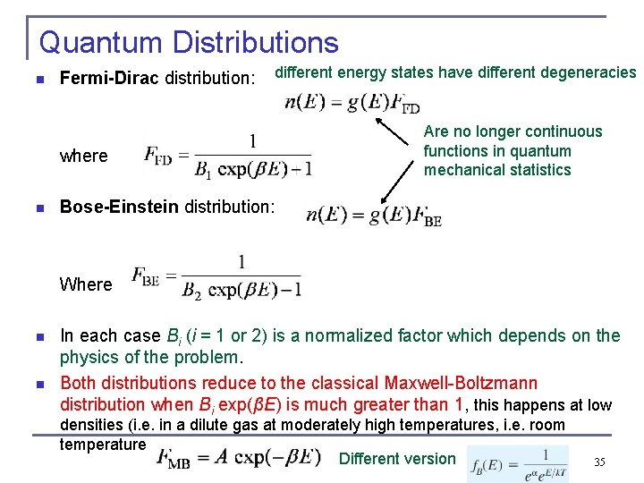
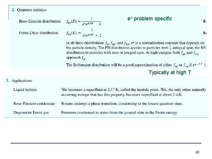
Quantum Distributions n Fermi-Dirac distribution: different energy states have different degeneracies where n Are no longer continuous functions in quantum mechanical statistics Bose-Einstein distribution: Where n n In each case Bi (i = 1 or 2) is a normalized factor which depends on the physics of the problem. Both distributions reduce to the classical Maxwell-Boltzmann distribution when Bi exp(βE) is much greater than 1, this happens at low densities (i. e. in a dilute gas at moderately high temperatures, i. e. room temperature Different version 35

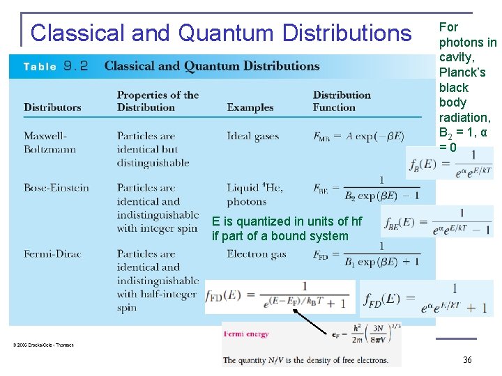
Classical and Quantum Distributions For photons in cavity, Planck’s black body radiation, B 2 = 1, α = 0 E is quantized in units of hf if part of a bound system 36

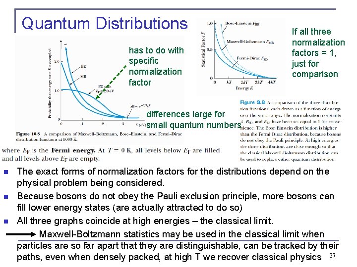
Quantum Distributions has to do with specific normalization factor If all three normalization factors = 1, just for comparison differences large for small quantum numbers n n n The exact forms of normalization factors for the distributions depend on the physical problem being considered. Because bosons do not obey the Pauli exclusion principle, more bosons can fill lower energy states (are actually attracted to do so) All three graphs coincide at high energies – the classical limit. Maxwell-Boltzmann statistics may be used in the classical limit when particles are so far apart that they are distinguishable, can be tracked by their paths, even when densely packed, at high T we recover classical physics 37

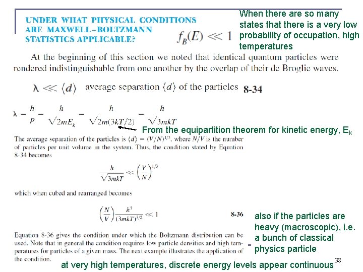
When there are so many states that there is a very low probability of occupation, high temperatures From the equipartition theorem for kinetic energy, Ek also if the particles are heavy (macroscopic), i. e. a bunch of classical physics particle at very high temperatures, discrete energy levels appear continuous 38

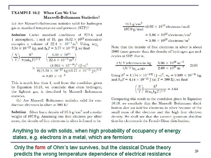
Anything to do with solids, when high probability of occupancy of energy states, e. g. electrons in a metal, which are fermions Only the form of Ohm’s law survives, but the classical Drude theory predicts the wrong temperature dependence of electrical resistance 39

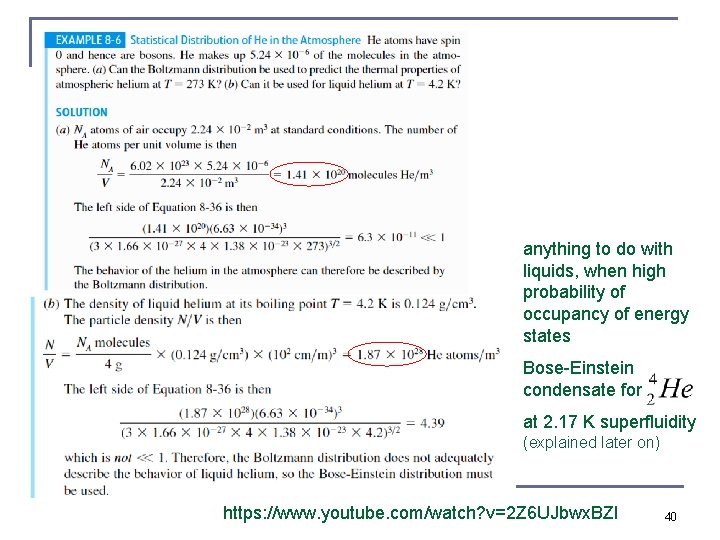
anything to do with liquids, when high probability of occupancy of energy states Bose-Einstein condensate for at 2. 17 K superfluidity (explained later on) https: //www. youtube. com/watch? v=2 Z 6 UJbwx. BZI 40

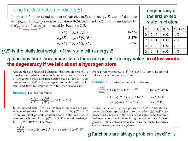
degeneracy of the first exited state in H atom g(E) is the statistical weight of the state with energy E n l ml ms up ms down 2 0 0 +1/2 -1/2 2 1 1 +1/2 -1/2 2 1 0 +1/2 -1/2 2 1 -1 +1/2 -1/2 g functions here: how many states there are per unit energy value, in other words: the degeneracy if we talk about a hydrogen atom g functions are always problem specific ! 41

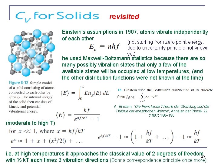
revisited Einstein’s assumptions in 1907, atoms vibrate independently of each other (not starting from zero point energy, due to uncertainty principle not known yet) he used Maxwell-Boltzmann statistics because there are so many possibly vibration states that only a few of the available states will be occupied at low temperatures, (and the other distribution functions were not known at the time) A. Einstein, "Die Plancksche Theorie der Strahlung und die Theorie der spezifischen Wärme", Annalen der Physik 22 (1907) 180– 190 (moderate to high T) i. e. at high temperatures it approaches the classical value of 2 degrees of freedom 42 with ½ k. T each times 3 vibration directions (Bohr’s correspondence principle once more)

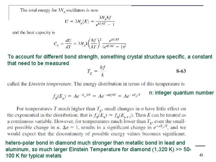
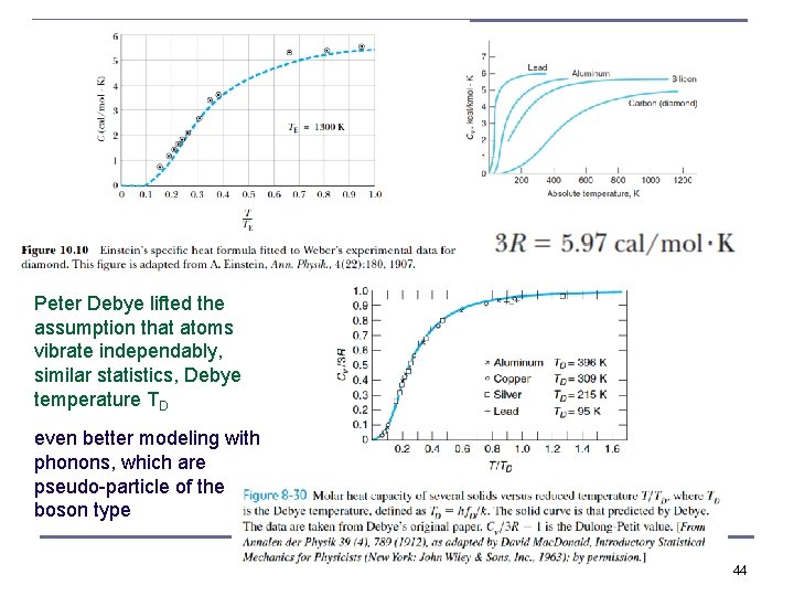
To account for different bond strength, something crystal structure specific, a constant that need to be measured n: integer quantum number hetero-polar bond in diamond much stronger than metallic bond in lead and aluminum, so much larger Einstein Temperature for diamond (1, 320 K) >> 50100 K for typical metals 43

Peter Debye lifted the assumption that atoms vibrate independably, similar statistics, Debye temperature TD even better modeling with phonons, which are pseudo-particle of the boson type 44

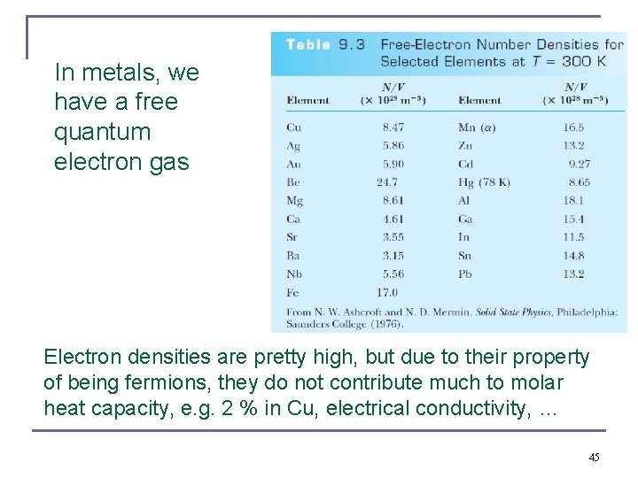
In metals, we have a free quantum electron gas Electron densities are pretty high, but due to their property of being fermions, they do not contribute much to molar heat capacity, e. g. 2 % in Cu, electrical conductivity, … 45

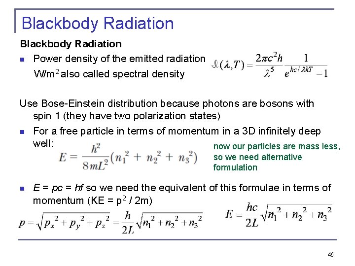
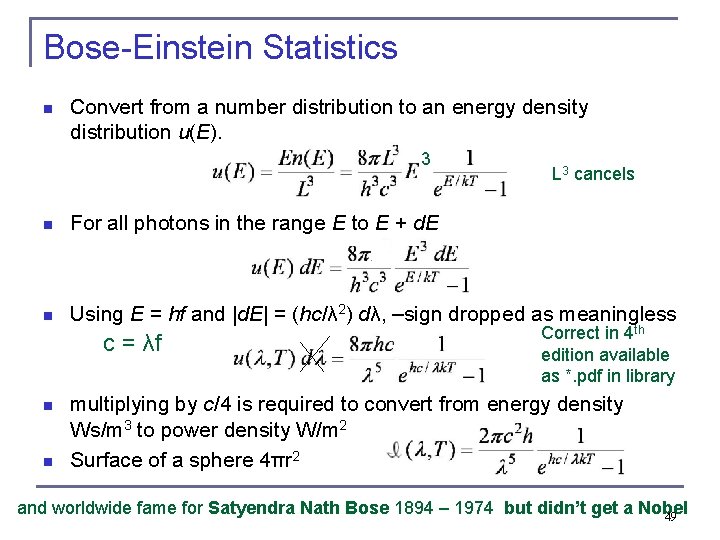
Blackbody Radiation n Power density of the emitted radiation W/m 2 also called spectral density Use Bose-Einstein distribution because photons are bosons with spin 1 (they have two polarization states) n For a free particle in terms of momentum in a 3 D infinitely deep well: now our particles are mass less, so we need alternative formulation n E = pc = hf so we need the equivalent of this formulae in terms of momentum (KE = p 2 / 2 m) 46

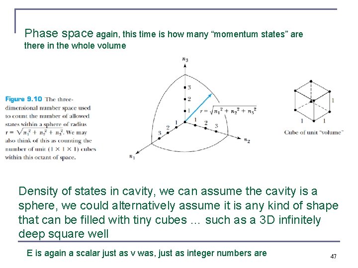
Phase space again, this time is how many “momentum states” are there in the whole volume Density of states in cavity, we can assume the cavity is a sphere, we could alternatively assume it is any kind of shape that can be filled with tiny cubes … such as a 3 D infinitely deep square well E is again a scalar just as v was, just as integer numbers are 47

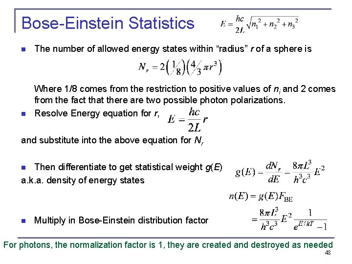
Bose-Einstein Statistics n The number of allowed energy states within “radius” r of a sphere is n Where 1/8 comes from the restriction to positive values of ni and 2 comes from the fact that there are two possible photon polarizations. Resolve Energy equation for r, and substitute into the above equation for Nr Then differentiate to get statistical weight g(E) a. k. a. density of energy states n n Multiply in Bose-Einstein distribution factor For photons, the normalization factor is 1, they are created and destroyed as needed 48

Bose-Einstein Statistics n Convert from a number distribution to an energy density distribution u(E). 3 L 3 cancels n For all photons in the range E to E + d. E n Using E = hf and |d. E| = (hc/λ 2) dλ, –sign dropped as meaningless c = λf n n Correct in 4 th edition available as *. pdf in library multiplying by c/4 is required to convert from energy density Ws/m 3 to power density W/m 2 Surface of a sphere 4πr 2 and worldwide fame for Satyendra Nath Bose 1894 – 1974 but didn’t get a Nobel 49

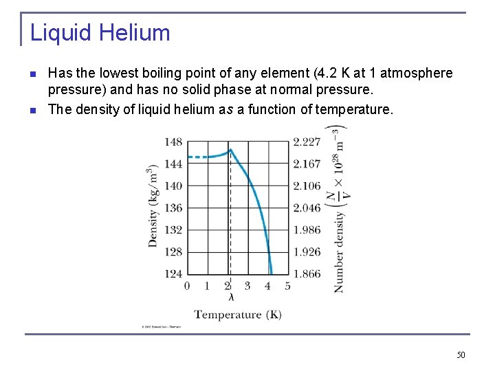
Liquid Helium n n Has the lowest boiling point of any element (4. 2 K at 1 atmosphere pressure) and has no solid phase at normal pressure. The density of liquid helium as a function of temperature. 50

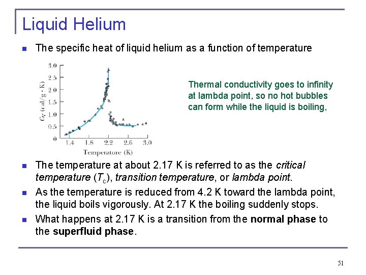
Liquid Helium n The specific heat of liquid helium as a function of temperature Thermal conductivity goes to infinity at lambda point, so no hot bubbles can form while the liquid is boiling, n n n The temperature at about 2. 17 K is referred to as the critical temperature (Tc), transition temperature, or lambda point. As the temperature is reduced from 4. 2 K toward the lambda point, the liquid boils vigorously. At 2. 17 K the boiling suddenly stops. What happens at 2. 17 K is a transition from the normal phase to the superfluid phase. 51

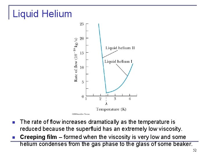
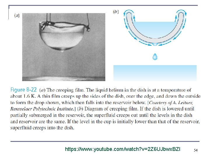
Liquid Helium n n The rate of flow increases dramatically as the temperature is reduced because the superfluid has an extremely low viscosity. Creeping film – formed when the viscosity is very low and some helium condenses from the gas phase to the glass of some beaker. 52

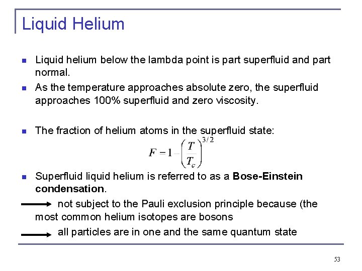
Liquid Helium n n Liquid helium below the lambda point is part superfluid and part normal. As the temperature approaches absolute zero, the superfluid approaches 100% superfluid and zero viscosity. n The fraction of helium atoms in the superfluid state: n Superfluid liquid helium is referred to as a Bose-Einstein condensation. not subject to the Pauli exclusion principle because (the most common helium isotopes are bosons all particles are in one and the same quantum state 53

https: //www. youtube. com/watch? v=2 Z 6 UJbwx. BZI 54

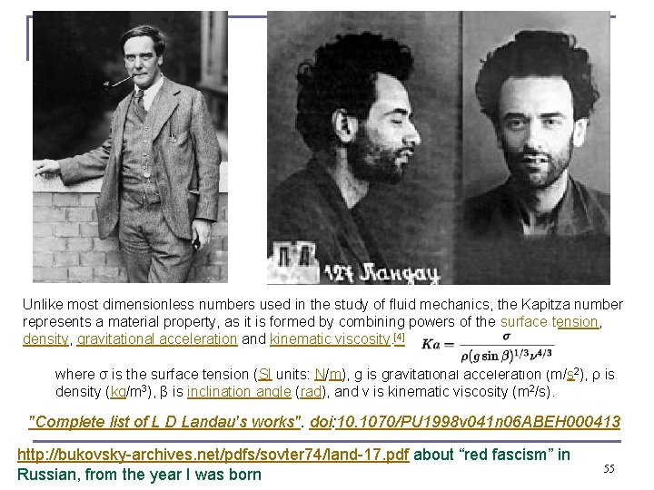
Unlike most dimensionless numbers used in the study of fluid mechanics, the Kapitza number represents a material property, as it is formed by combining powers of the surface tension, density, gravitational acceleration and kinematic viscosity. [4] where σ is the surface tension (SI units: N/m), g is gravitational acceleration (m/s 2), ρ is density (kg/m 3), β is inclination angle (rad), and ν is kinematic viscosity (m 2/s). "Complete list of L D Landau's works". doi: 10. 1070/PU 1998 v 041 n 06 ABEH 000413 http: //bukovsky-archives. net/pdfs/sovter 74/land-17. pdf about “red fascism” in Russian, from the year I was born 55

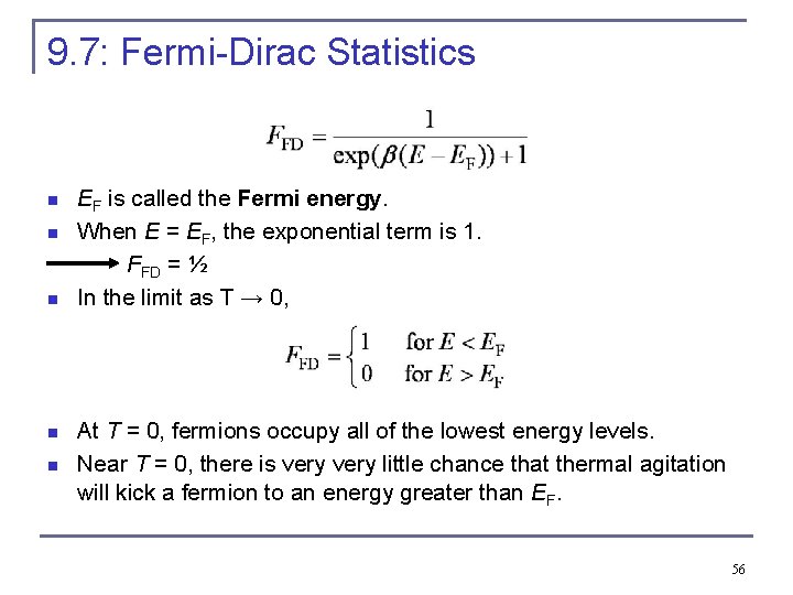
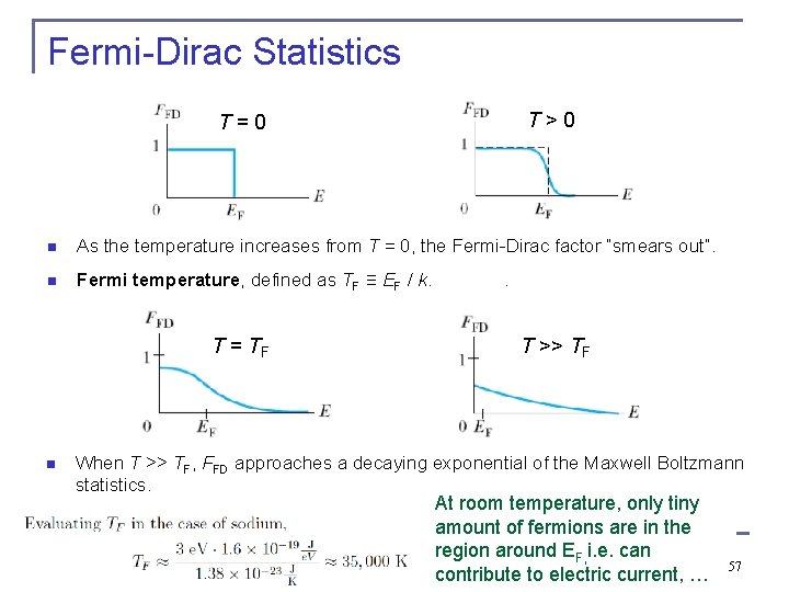
9. 7: Fermi-Dirac Statistics n n n EF is called the Fermi energy. When E = EF, the exponential term is 1. FFD = ½ In the limit as T → 0, At T = 0, fermions occupy all of the lowest energy levels. Near T = 0, there is very little chance that thermal agitation will kick a fermion to an energy greater than EF. 56

Fermi-Dirac Statistics T > 0 T = 0 n As the temperature increases from T = 0, the Fermi-Dirac factor “smears out”. n Fermi temperature, defined as TF ≡ EF / k. . T = TF n T >> TF When T >> TF, FFD approaches a decaying exponential of the Maxwell Boltzmann statistics. At room temperature, only tiny amount of fermions are in the region around EF, i. e. can contribute to electric current, … 57

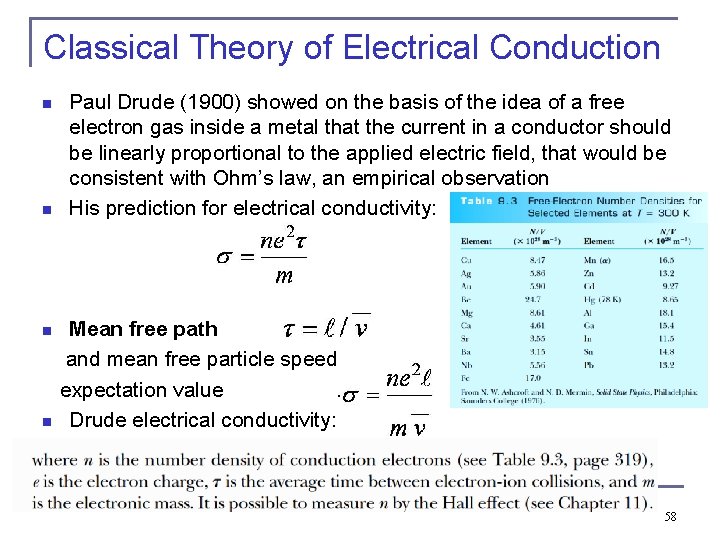
Classical Theory of Electrical Conduction n n Paul Drude (1900) showed on the basis of the idea of a free electron gas inside a metal that the current in a conductor should be linearly proportional to the applied electric field, that would be consistent with Ohm’s law, an empirical observation His prediction for electrical conductivity: Mean free path and mean free particle speed expectation value . n Drude electrical conductivity: n 58

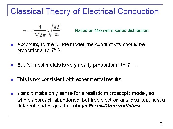
Classical Theory of Electrical Conduction Based on Maxwell’s speed distribution n According to the Drude model, the conductivity should be proportional to T− 1/2. n But for most metals is very nearly proportional to T− 1 !! n This is not consistent with experimental results. n l and τ make only sense for a realistic microscopic model, so whole approach abandoned, but free electron gas idea kept, just a different kind of gas that obeys Fermi-Dirac statistics 59

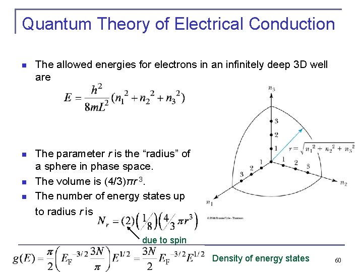
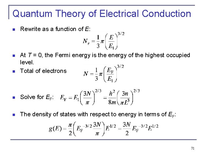
Quantum Theory of Electrical Conduction n The allowed energies for electrons in an infinitely deep 3 D well are n The parameter r is the “radius” of a sphere in phase space. The volume is (4/3)πr 3. The number of energy states up to radius r is . n n due to spin Density of energy states 60

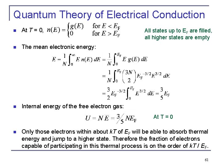
Quantum Theory of Electrical Conduction n At T = 0, n The mean electronic energy: n Internal energy of the free electron gas: All states up to EF are filled, all higher states are empty At T = 0 n Only those electrons within about k. T of EF will be able to absorb thermal energy and jump to a higher state. Therefore the fraction of electrons capable of participating in this thermal process is on the order of k. T / EF. 61

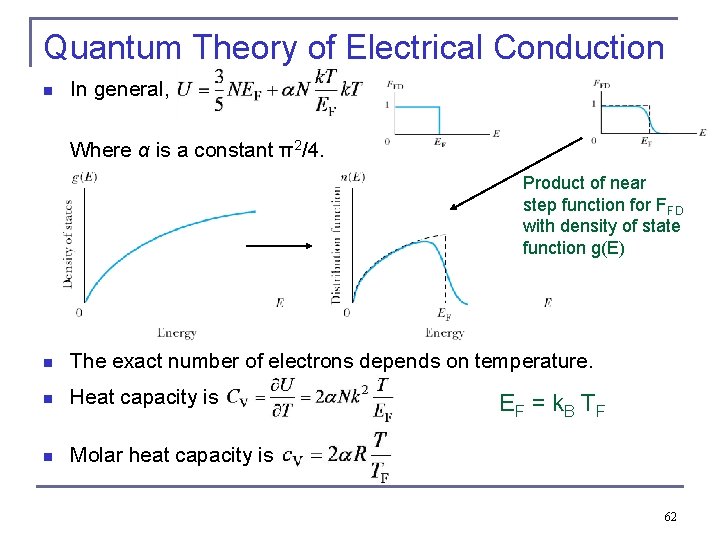
Quantum Theory of Electrical Conduction n In general, Where α is a constant π2/4. Product of near step function for FFD with density of state function g(E) n The exact number of electrons depends on temperature. n Heat capacity is n Molar heat capacity is EF = k. B TF 62

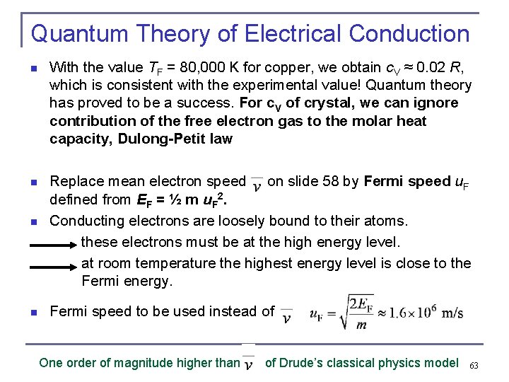
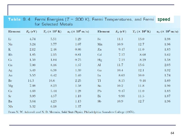
Quantum Theory of Electrical Conduction n With the value TF = 80, 000 K for copper, we obtain c. V ≈ 0. 02 R, which is consistent with the experimental value! Quantum theory has proved to be a success. For c. V of crystal, we can ignore contribution of the free electron gas to the molar heat capacity, Dulong-Petit law n Replace mean electron speed on slide 58 by Fermi speed u. F defined from EF = ½ m u. F 2. Conducting electrons are loosely bound to their atoms. these electrons must be at the high energy level. at room temperature the highest energy level is close to the Fermi energy. n n Fermi speed to be used instead of One order of magnitude higher than of Drude’s classical physics model 63

speed 64

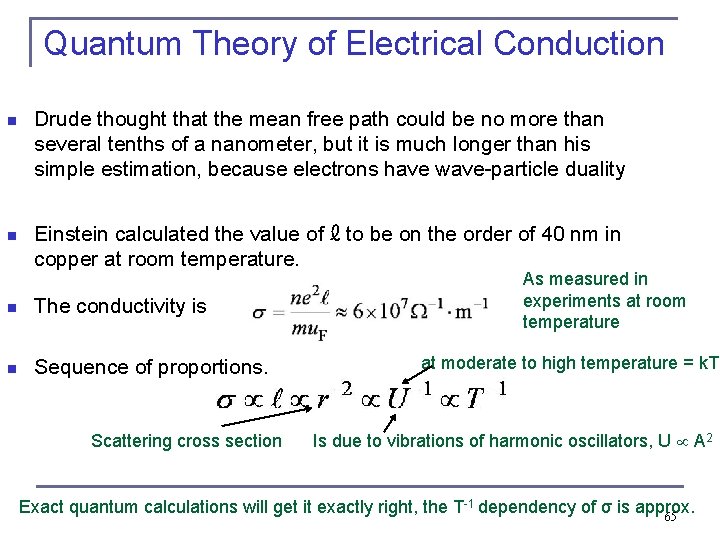
Quantum Theory of Electrical Conduction n n Drude thought that the mean free path could be no more than several tenths of a nanometer, but it is much longer than his simple estimation, because electrons have wave-particle duality Einstein calculated the value of ℓ to be on the order of 40 nm in copper at room temperature. n The conductivity is n Sequence of proportions. Scattering cross section As measured in experiments at room temperature at moderate to high temperature = k. T Is due to vibrations of harmonic oscillators, U A 2 Exact quantum calculations will get it exactly right, the T-1 dependency of σ is approx. 65

66

B for Boltzmann, also MB 67

eα problem specific >> Typically at high T 68

Change from Maxwell speed distribution to kinetic energy distribution n Rewrite Maxwell speed distribution in terms of energy. n For a monatomic gas the energy is all translational kinetic energy. where 69

statistical All condensed matter (liquids and solids) problems are statistical quantum mechanics problems !! Quantum condensed matter physics problems are typically low temperature problems Ideal gasses can be modeled classically, because they have very low matter densities 70

Quantum Theory of Electrical Conduction n Rewrite as a function of E: n n At T = 0, the Fermi energy is the energy of the highest occupied level. Total of electrons n Solve for EF: n The density of states with respect to energy in terms of EF: 71