Chapter 9 Slide 1 Correlation and Regression 9

Chapter 9 Slide 1 Correlation and Regression 9 -1 Overview 9 -2 Correlation 9 -3 Regression 9 -4 Variation and Prediction Intervals 9 -5 Multiple Regression 9 -6 Modeling Chapter 9, Triola, Elementary Statistics, MATH 1342

Slide 2 Section 9 -1 & 9 -2 Overview and Correlation and Regression Created by Erin Hodgess, Houston, Texas

Overview Slide 3 Paired Data (p. 506) v. Is there a relationship? v. If so, what is the equation? v. Use that equation for prediction. Chapter 9, Triola, Elementary Statistics, MATH 1342

Definition Slide 4 v. A correlation exists between two variables when one of them is related to the other in some way. Chapter 9, Triola, Elementary Statistics, MATH 1342

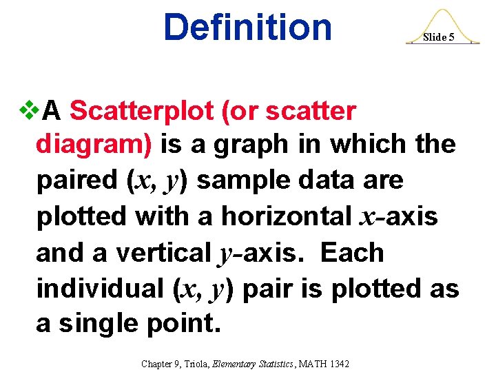
Definition Slide 5 v. A Scatterplot (or scatter diagram) is a graph in which the paired (x, y) sample data are plotted with a horizontal x-axis and a vertical y-axis. Each individual (x, y) pair is plotted as a single point. Chapter 9, Triola, Elementary Statistics, MATH 1342

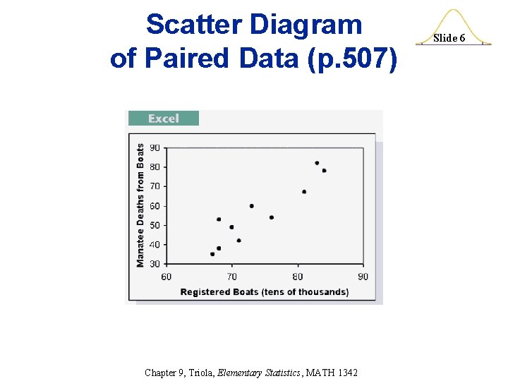
Scatter Diagram of Paired Data (p. 507) Chapter 9, Triola, Elementary Statistics, MATH 1342 Slide 6

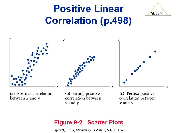
Positive Linear Correlation (p. 498) Figure 9 -2 Scatter Plots Chapter 9, Triola, Elementary Statistics, MATH 1342 Slide 7

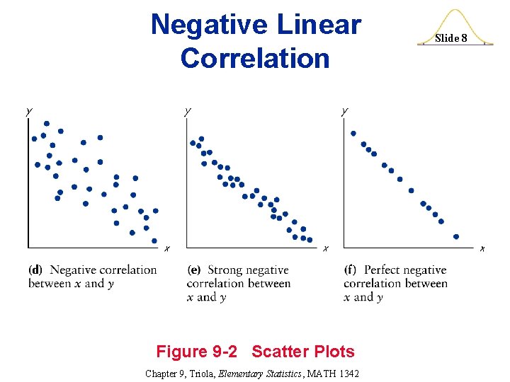
Negative Linear Correlation Figure 9 -2 Scatter Plots Chapter 9, Triola, Elementary Statistics, MATH 1342 Slide 8

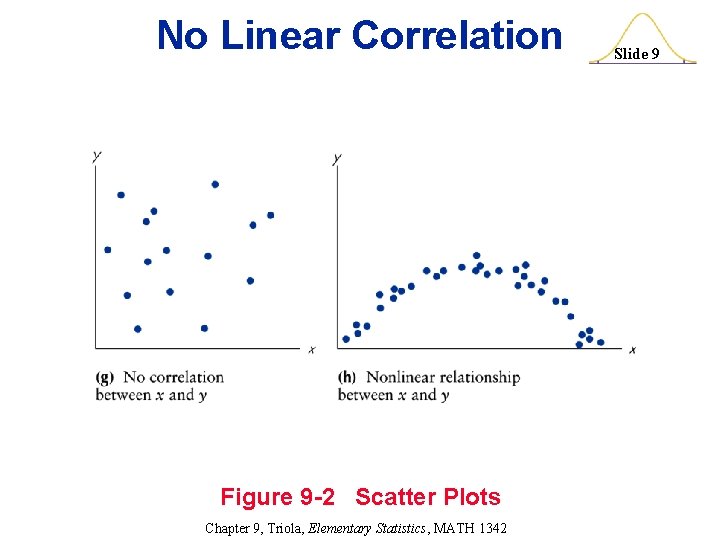
No Linear Correlation Figure 9 -2 Scatter Plots Chapter 9, Triola, Elementary Statistics, MATH 1342 Slide 9

Definition (p. 509) Slide 10 The linear correlation coefficient r measures strength of the linear relationship between paired x and y values in a sample. Chapter 9, Triola, Elementary Statistics, MATH 1342

Assumptions (p. 507) Slide 11 1. The sample of paired data (x, y) is a random sample. 2. The pairs of (x, y) data have a bivariate normal distribution. Chapter 9, Triola, Elementary Statistics, MATH 1342

Notation for the Linear Correlation Coefficient Slide 12 n = number of pairs of data presented denotes the addition of the items indicated. x denotes the sum of all x-values. x 2 indicates that each x-value should be squared and then those squares added. ( x)2 indicates that the x-values should be added and the total then squared. xy indicates that each x-value should be first multiplied by its corresponding y-value. After obtaining all such products, find their sum. r represents linear correlation coefficient for a sample represents linear correlation coefficient for a population Chapter 9, Triola, Elementary Statistics, MATH 1342

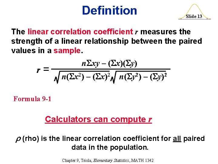
Definition Slide 13 The linear correlation coefficient r measures the strength of a linear relationship between the paired values in a sample. r= n xy – ( x)( y) n( x 2) – ( x)2 n( y 2) – ( y)2 Formula 9 -1 Calculators can compute r (rho) is the linear correlation coefficient for all paired data in the population. Chapter 9, Triola, Elementary Statistics, MATH 1342

Rounding the Linear Correlation Coefficient r Slide 14 v Round to three decimal places so that it can be compared to critical values in Table A-6. (see p. 510) v Use calculator or computer if possible. Chapter 9, Triola, Elementary Statistics, MATH 1342

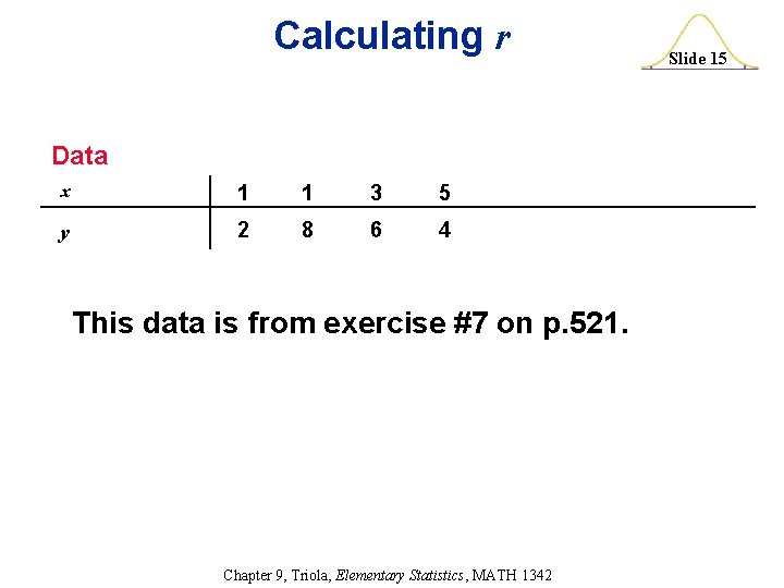
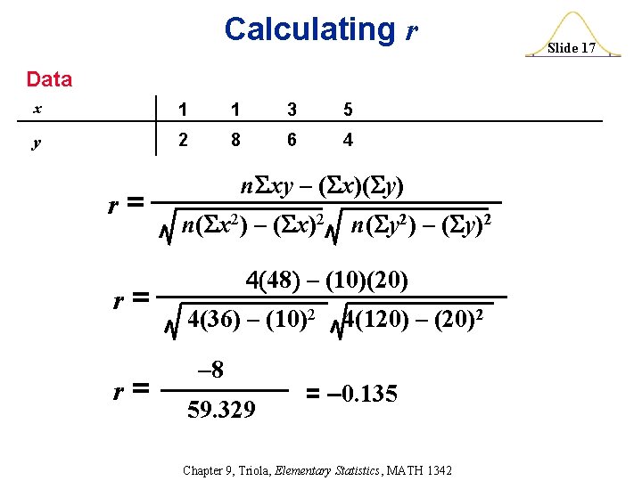
Calculating r Data x 1 1 3 5 y 2 8 6 4 This data is from exercise #7 on p. 521. Chapter 9, Triola, Elementary Statistics, MATH 1342 Slide 15

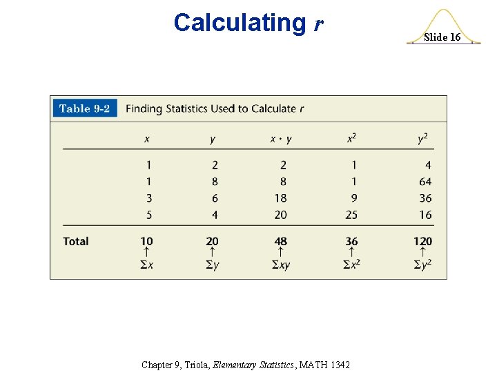
Calculating r Chapter 9, Triola, Elementary Statistics, MATH 1342 Slide 16

Calculating r Data x 1 1 3 5 y 2 8 6 4 r= r= r= n xy – ( x)( y) n( x 2) – ( x)2 n( y 2) – ( y)2 4(48) – (10)(20) 4(36) – (10)2 – 8 59. 329 4(120) – (20)2 = – 0. 135 Chapter 9, Triola, Elementary Statistics, MATH 1342 Slide 17

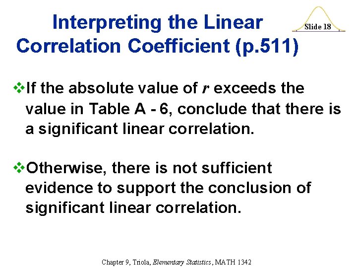
Interpreting the Linear Correlation Coefficient (p. 511) Slide 18 v. If the absolute value of r exceeds the value in Table A - 6, conclude that there is a significant linear correlation. v. Otherwise, there is not sufficient evidence to support the conclusion of significant linear correlation. Chapter 9, Triola, Elementary Statistics, MATH 1342

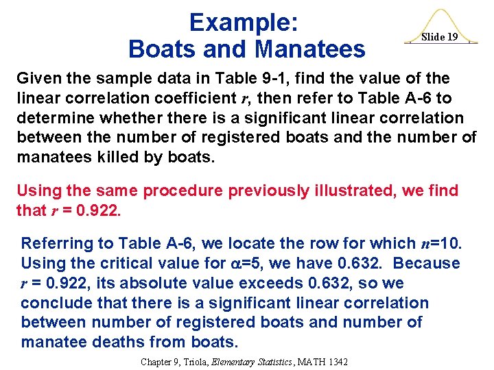
Example: Boats and Manatees Slide 19 Given the sample data in Table 9 -1, find the value of the linear correlation coefficient r, then refer to Table A-6 to determine whethere is a significant linear correlation between the number of registered boats and the number of manatees killed by boats. Using the same procedure previously illustrated, we find that r = 0. 922. Referring to Table A-6, we locate the row for which n=10. Using the critical value for =5, we have 0. 632. Because r = 0. 922, its absolute value exceeds 0. 632, so we conclude that there is a significant linear correlation between number of registered boats and number of manatee deaths from boats. Chapter 9, Triola, Elementary Statistics, MATH 1342

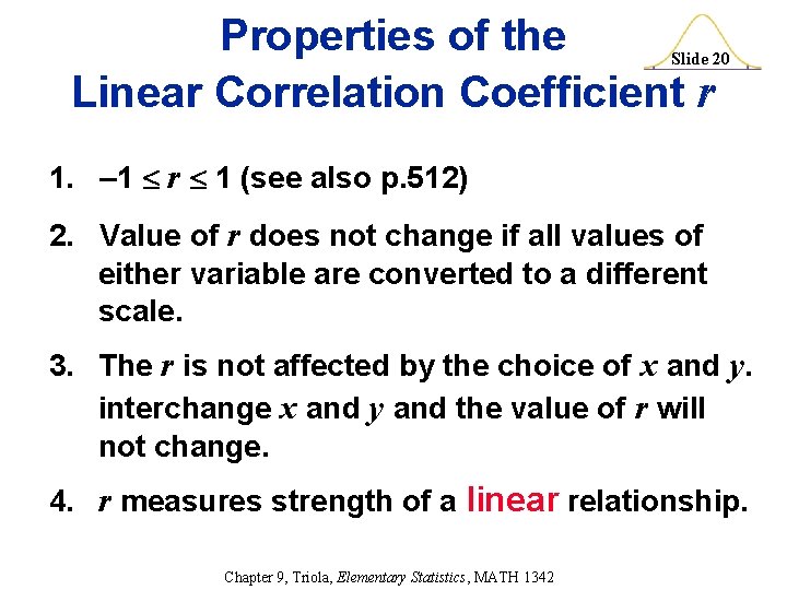
Properties of the Linear Correlation Coefficient r Slide 20 1. – 1 r 1 (see also p. 512) 2. Value of r does not change if all values of either variable are converted to a different scale. 3. The r is not affected by the choice of x and y. interchange x and y and the value of r will not change. 4. r measures strength of a linear relationship. Chapter 9, Triola, Elementary Statistics, MATH 1342

Interpreting r: Explained Variation Slide 21 The value of r 2 is the proportion of the variation in y that is explained by the linear relationship between x and y. (p. 503 and p. 533) Chapter 9, Triola, Elementary Statistics, MATH 1342

Example: Boats and Manatees Slide 22 Using the boat/manatee data in Table 9 -1, we have found that the value of the linear correlation coefficient r = 0. 922. What proportion of the variation of the manatee deaths can be explained by the variation in the number of boat registrations? With r = 0. 922, we get r 2 = 0. 850. We conclude that 0. 850 (or about 85%) of the variation in manatee deaths can be explained by the linear relationship between the number of boat registrations and the number of manatee deaths from boats. This implies that 15% of the variation of manatee deaths cannot be explained by the number of boat registrations. Chapter 9, Triola, Elementary Statistics, MATH 1342

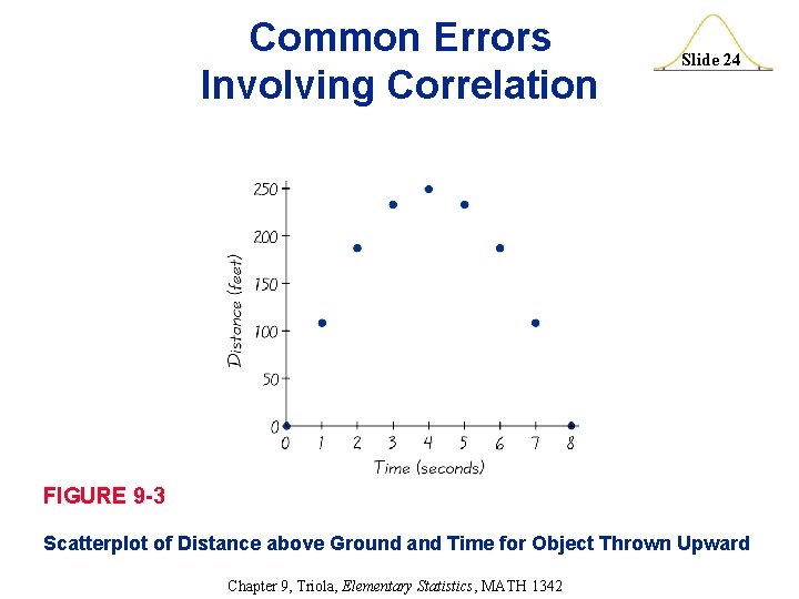
Common Errors Involving Correlation (pp. 503 -504) Slide 23 1. Causation: It is wrong to conclude that correlation implies causality. 2. Averages: Averages suppress individual variation and may inflate the correlation coefficient. 3. Linearity: There may be some relationship between x and y even when there is no significant linear correlation. Chapter 9, Triola, Elementary Statistics, MATH 1342

Common Errors Involving Correlation Slide 24 FIGURE 9 -3 Scatterplot of Distance above Ground and Time for Object Thrown Upward Chapter 9, Triola, Elementary Statistics, MATH 1342

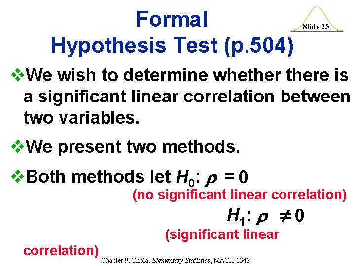
Formal Hypothesis Test (p. 504) Slide 25 v. We wish to determine whethere is a significant linear correlation between two variables. v. We present two methods. v. Both methods let H 0: = (no significant linear correlation) H 1: (significant linear correlation) Chapter 9, Triola, Elementary Statistics, MATH 1342

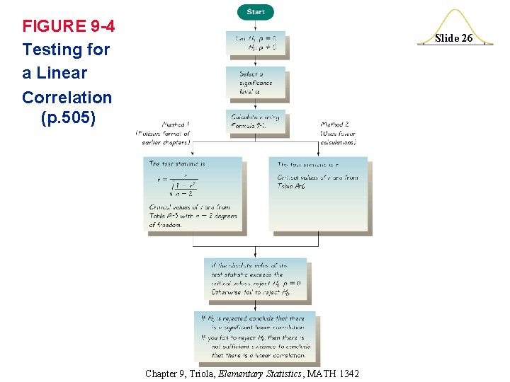
FIGURE 9 -4 Testing for a Linear Correlation (p. 505) Slide 26 Chapter 9, Triola, Elementary Statistics, MATH 1342

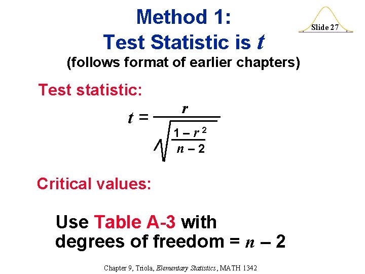
Method 1: Test Statistic is t (follows format of earlier chapters) Test statistic: t= r 1 – r 2 n – 2 Critical values: Use Table A-3 with degrees of freedom = n – 2 Chapter 9, Triola, Elementary Statistics, MATH 1342 Slide 27

Method 2: Test Statistic is r (uses fewer calculations) v. Test statistic: r v. Critical values: Refer to Table A-6 (no degrees of freedom) Chapter 9, Triola, Elementary Statistics, MATH 1342 Slide 28

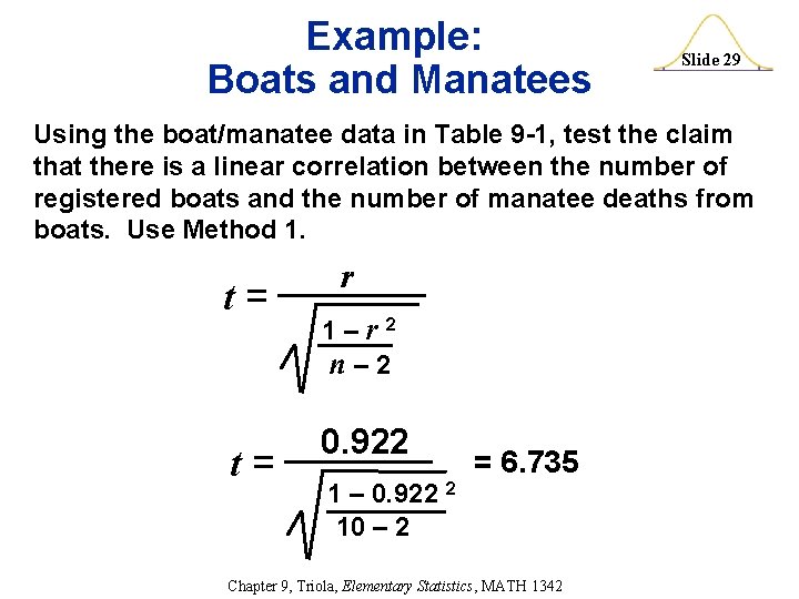
Example: Boats and Manatees Slide 29 Using the boat/manatee data in Table 9 -1, test the claim that there is a linear correlation between the number of registered boats and the number of manatee deaths from boats. Use Method 1. t= t= r 1 – r 2 n – 2 0. 922 1 – 0. 922 2 10 – 2 = 6. 735 Chapter 9, Triola, Elementary Statistics, MATH 1342

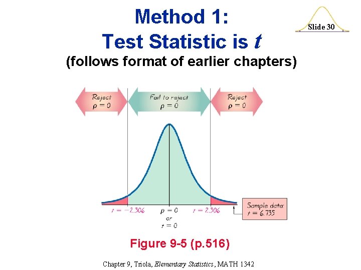
Method 1: Test Statistic is t (follows format of earlier chapters) Figure 9 -5 (p. 516) Chapter 9, Triola, Elementary Statistics, MATH 1342 Slide 30

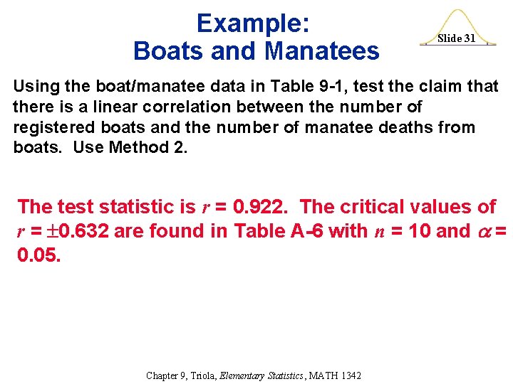
Example: Boats and Manatees Slide 31 Using the boat/manatee data in Table 9 -1, test the claim that there is a linear correlation between the number of registered boats and the number of manatee deaths from boats. Use Method 2. The test statistic is r = 0. 922. The critical values of r = 0. 632 are found in Table A-6 with n = 10 and = 0. 05. Chapter 9, Triola, Elementary Statistics, MATH 1342

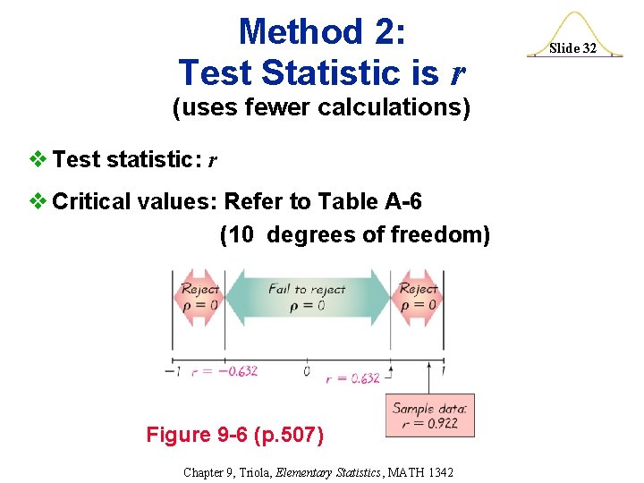
Method 2: Test Statistic is r (uses fewer calculations) v Test statistic: r v Critical values: Refer to Table A-6 (10 degrees of freedom) Figure 9 -6 (p. 507) Chapter 9, Triola, Elementary Statistics, MATH 1342 Slide 32

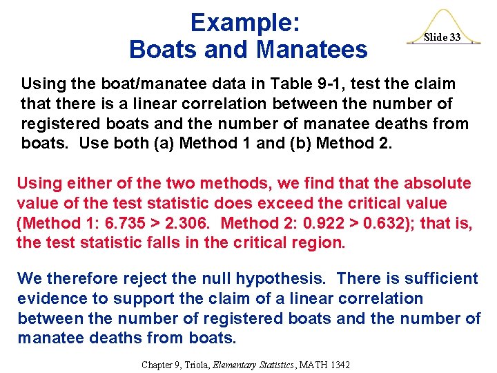
Example: Boats and Manatees Slide 33 Using the boat/manatee data in Table 9 -1, test the claim that there is a linear correlation between the number of registered boats and the number of manatee deaths from boats. Use both (a) Method 1 and (b) Method 2. Using either of the two methods, we find that the absolute value of the test statistic does exceed the critical value (Method 1: 6. 735 > 2. 306. Method 2: 0. 922 > 0. 632); that is, the test statistic falls in the critical region. We therefore reject the null hypothesis. There is sufficient evidence to support the claim of a linear correlation between the number of registered boats and the number of manatee deaths from boats. Chapter 9, Triola, Elementary Statistics, MATH 1342

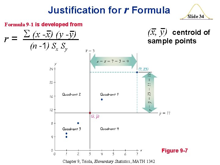
Justification for r Formula 9 -1 is developed from (x -x) (y -y) r = (n -1) Sx Sy Slide 34 (x, y) centroid of sample points Figure 9 -7 Chapter 9, Triola, Elementary Statistics, MATH 1342

Slide 35 Section 9 -3 Regression Created by Erin Hodgess, Houston, Texas

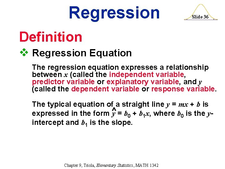
Regression Slide 36 Definition v Regression Equation The regression equation expresses a relationship between x (called the independent variable, predictor variable or explanatory variable, and y (called the dependent variable or response variable. The typical equation of a straight line y = mx + b is ^ 0 + b 1 x, where b 0 is the yexpressed in the form y = b intercept and b 1 is the slope. Chapter 9, Triola, Elementary Statistics, MATH 1342

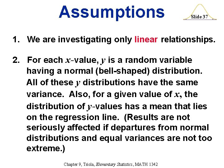
Assumptions Slide 37 1. We are investigating only linear relationships. 2. For each x-value, y is a random variable having a normal (bell-shaped) distribution. All of these y distributions have the same variance. Also, for a given value of x, the distribution of y-values has a mean that lies on the regression line. (Results are not seriously affected if departures from normal distributions and equal variances are not too extreme. ) Chapter 9, Triola, Elementary Statistics, MATH 1342

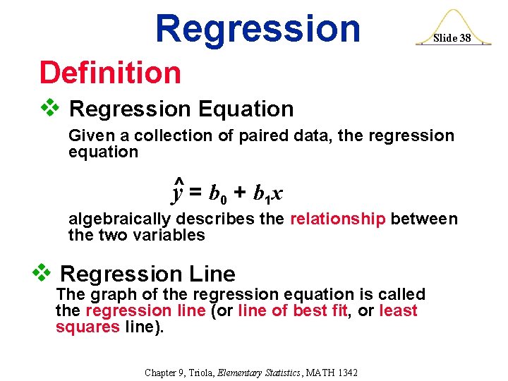
Regression Slide 38 Definition v Regression Equation Given a collection of paired data, the regression equation y^ = b 0 + b 1 x algebraically describes the relationship between the two variables v Regression Line The graph of the regression equation is called the regression line (or line of best fit, or least squares line). Chapter 9, Triola, Elementary Statistics, MATH 1342

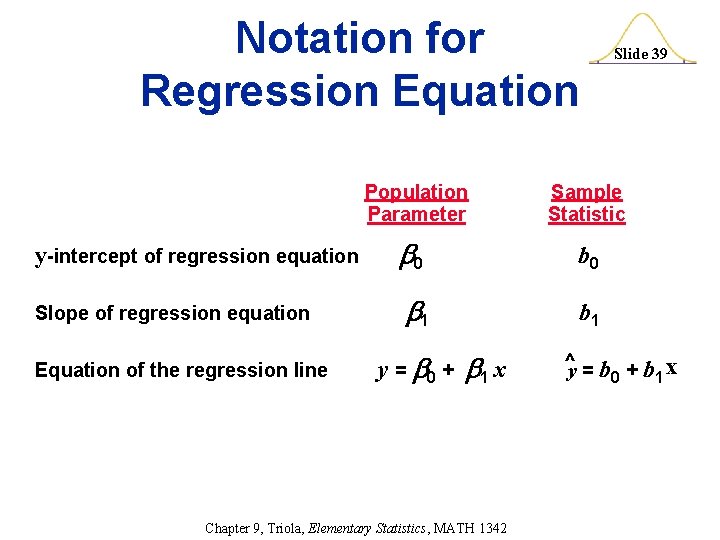
Notation for Regression Equation Population Parameter Slide 39 Sample Statistic y-intercept of regression equation 0 b 0 Slope of regression equation 1 b 1 Equation of the regression line y = 0 + 1 x ^y = b 0 + b 1 x Chapter 9, Triola, Elementary Statistics, MATH 1342

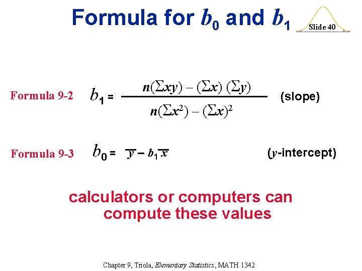
Formula for b 0 and b 1 Slide 40 n( xy) – ( x) ( y) Formula 9 -2 b 1 = Formula 9 -3 b 0 = y – b 1 x (y-intercept) (slope) n( x 2) – ( x)2 calculators or computers can compute these values Chapter 9, Triola, Elementary Statistics, MATH 1342

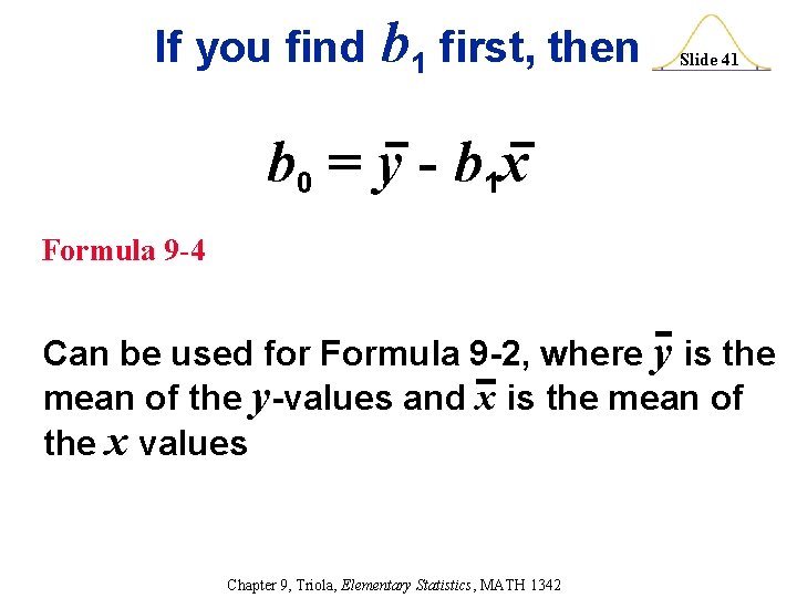
If you find b 1 first, then Slide 41 b 0 = y - b 1 x Formula 9 -4 Can be used for Formula 9 -2, where y is the mean of the y-values and x is the mean of the x values Chapter 9, Triola, Elementary Statistics, MATH 1342

Slide 42 The regression line fits the sample points best. Chapter 9, Triola, Elementary Statistics, MATH 1342

Rounding the y-intercept b 0 and the slope b 1 Slide 43 v Round to three significant digits. v If you use the formulas 9 -2 and 9 -3, try not to round intermediate values. (see p. 527) Chapter 9, Triola, Elementary Statistics, MATH 1342

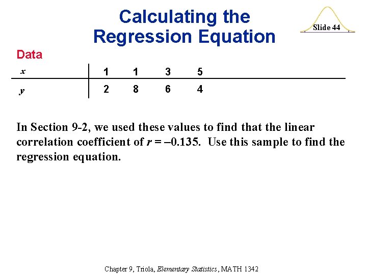
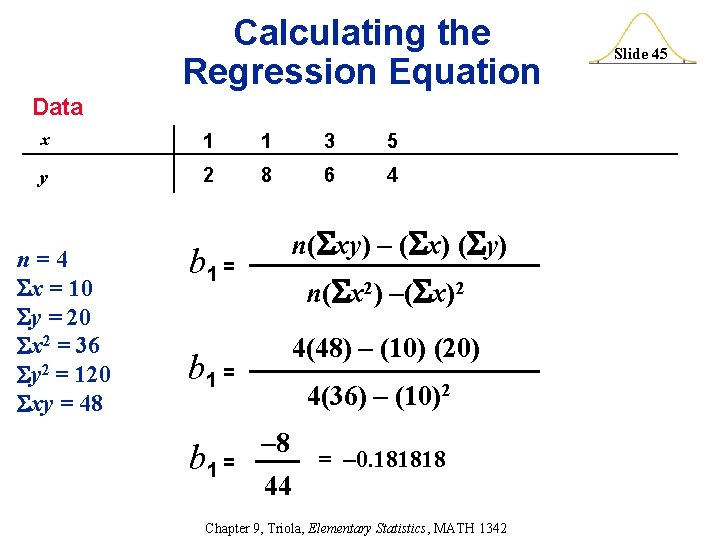
Calculating the Regression Equation Slide 44 Data x 1 1 3 5 y 2 8 6 4 In Section 9 -2, we used these values to find that the linear correlation coefficient of r = – 0. 135. Use this sample to find the regression equation. Chapter 9, Triola, Elementary Statistics, MATH 1342

Calculating the Regression Equation Data x 1 1 3 5 y 2 8 6 4 n=4 x = 10 y = 20 x 2 = 36 y 2 = 120 xy = 48 n( xy) – ( x) ( y) b 1 = n( x 2) –( x)2 4(48) – (10) (20) b 1 = 4(36) – (10)2 – 8 44 = – 0. 181818 Chapter 9, Triola, Elementary Statistics, MATH 1342 Slide 45

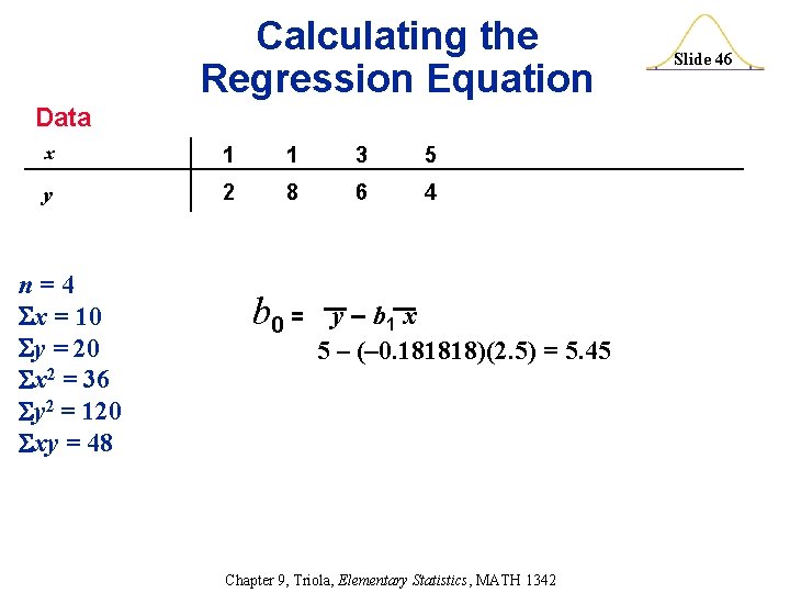
Calculating the Regression Equation Data x 1 1 3 5 y 2 8 6 4 n=4 x = 10 y = 20 x 2 = 36 y 2 = 120 xy = 48 b 0 = y – b 1 x 5 – (– 0. 181818)(2. 5) = 5. 45 Chapter 9, Triola, Elementary Statistics, MATH 1342 Slide 46

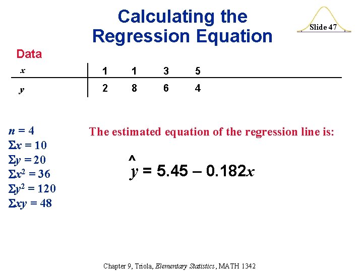
Calculating the Regression Equation Slide 47 Data x 1 1 3 5 y 2 8 6 4 n=4 x = 10 y = 20 x 2 = 36 y 2 = 120 xy = 48 The estimated equation of the regression line is: ^ y = 5. 45 – 0. 182 x Chapter 9, Triola, Elementary Statistics, MATH 1342

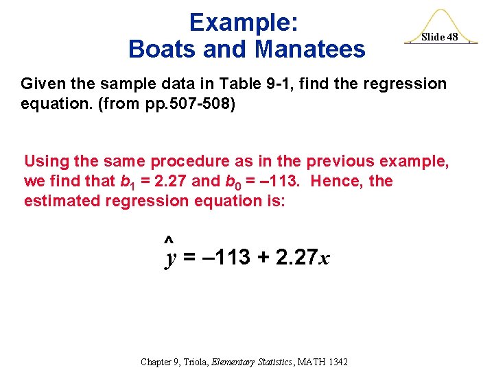
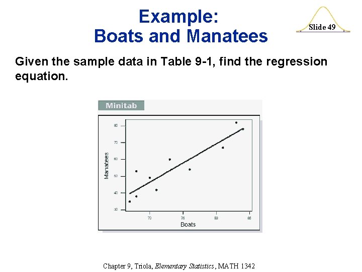
Example: Boats and Manatees Slide 48 Given the sample data in Table 9 -1, find the regression equation. (from pp. 507 -508) Using the same procedure as in the previous example, we find that b 1 = 2. 27 and b 0 = – 113. Hence, the estimated regression equation is: ^ y = – 113 + 2. 27 x Chapter 9, Triola, Elementary Statistics, MATH 1342

Example: Boats and Manatees Slide 49 Given the sample data in Table 9 -1, find the regression equation. Chapter 9, Triola, Elementary Statistics, MATH 1342

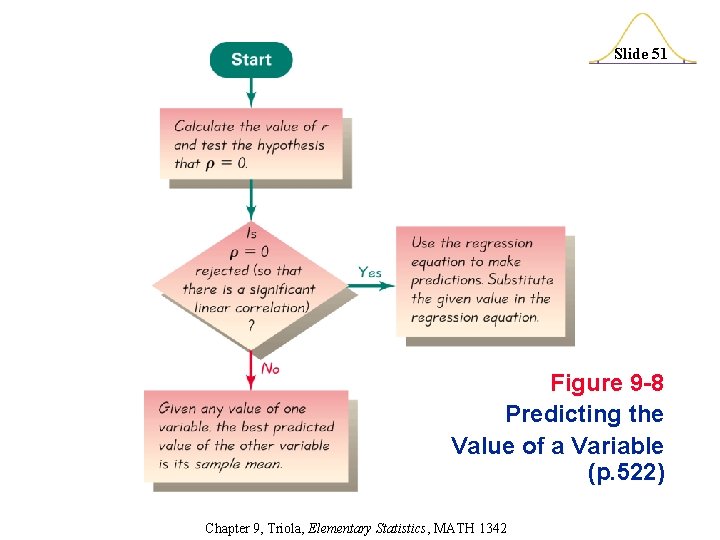
Predictions Slide 50 In predicting a value of y based on some given value of x. . . 1. If there is not a significant linear correlation, the best predicted y-value is y. 2. If there is a significant linear correlation, the best predicted y-value is found by substituting the x-value into the regression equation. Chapter 9, Triola, Elementary Statistics, MATH 1342

Slide 51 Figure 9 -8 Predicting the Value of a Variable (p. 522) Chapter 9, Triola, Elementary Statistics, MATH 1342

Example: Boats and Manatees Slide 52 Given the sample data in Table 9 -1, we found that the ^ regression equation is y = – 113 + 2. 27 x. Assume that in 2001 there were 850, 000 registered boats. Because Table 9 -1 lists the numbers of registered boats in tens of thousands, this means that for 2001 we have x = 85. Given that x = 85, find the best predicted value of y, the number of manatee deaths from boats. Chapter 9, Triola, Elementary Statistics, MATH 1342

Example: Boats and Manatees Slide 53 Given the sample data in Table 9 -1, we found that the ^ regression equation is y = – 113 + 2. 27 x. Given that x = 85, find the best predicted value of y, the number of manatee deaths from boats. We must consider whethere is a linear correlation that justifies the use of that equation. We do have a significant linear correlation (with r = 0. 922). Chapter 9, Triola, Elementary Statistics, MATH 1342

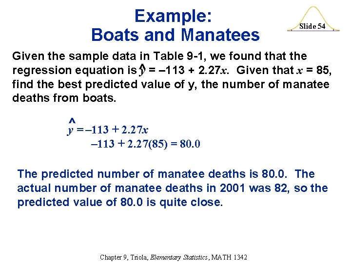
Example: Boats and Manatees Slide 54 Given the sample data in Table 9 -1, we found that the ^ regression equation is y = – 113 + 2. 27 x. Given that x = 85, find the best predicted value of y, the number of manatee deaths from boats. ^ y = – 113 + 2. 27 x – 113 + 2. 27(85) = 80. 0 The predicted number of manatee deaths is 80. 0. The actual number of manatee deaths in 2001 was 82, so the predicted value of 80. 0 is quite close. Chapter 9, Triola, Elementary Statistics, MATH 1342

Guidelines for Using The Regression Equation (p. 523) Slide 55 1. If there is no significant linear correlation, don’t use the regression equation to make predictions. 2. When using the regression equation for predictions, stay within the scope of the available sample data. 3. A regression equation based on old data is not necessarily valid now. 4. Don’t make predictions about a population that is different from the population from which the sample data was drawn. Chapter 9, Triola, Elementary Statistics, MATH 1342

Definitions Slide 56 v Marginal Change: The marginal change is the amount that a variable changes when the other variable changes by exactly one unit. v Outlier: An outlier is a point lying far away from the other data points. v Influential Points: An influential point strongly affects the graph of the regression line. Chapter 9, Triola, Elementary Statistics, MATH 1342

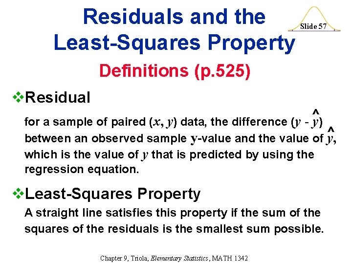
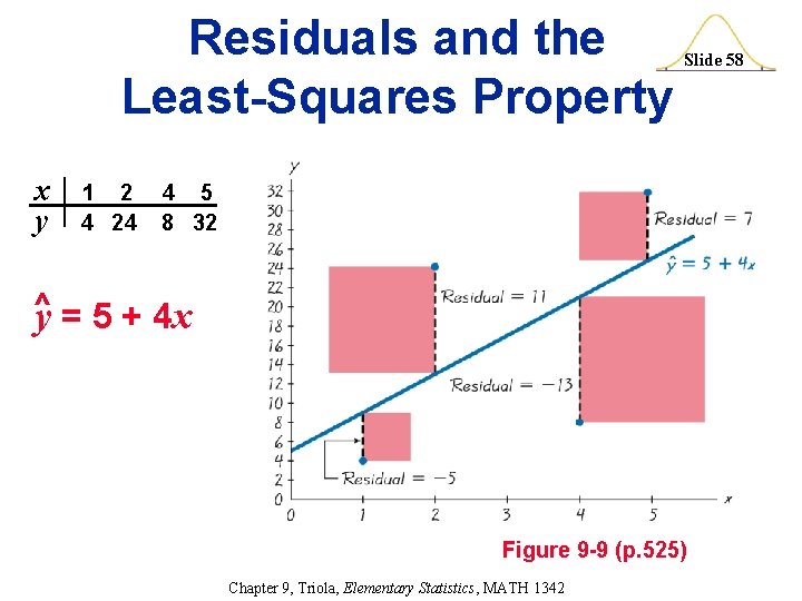
Residuals and the Least-Squares Property Slide 57 Definitions (p. 525) v. Residual ^ for a sample of paired (x, y) data, the difference (y - y) between an observed sample y-value and the value of ^ y, which is the value of y that is predicted by using the regression equation. v. Least-Squares Property A straight line satisfies this property if the sum of the squares of the residuals is the smallest sum possible. Chapter 9, Triola, Elementary Statistics, MATH 1342

Residuals and the Least-Squares Property Slide 58 x 1 2 4 5 y 4 24 8 32 ^ y = 5 + 4 x Figure 9 -9 (p. 525) Chapter 9, Triola, Elementary Statistics, MATH 1342

Slide 59 Section 9 -4 Variation and Prediction Intervals Created by Erin Hodgess, Houston, Texas

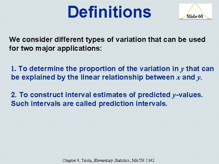
Definitions Slide 60 We consider different types of variation that can be used for two major applications: 1. To determine the proportion of the variation in y that can be explained by the linear relationship between x and y. 2. To construct interval estimates of predicted y-values. Such intervals are called prediction intervals. Chapter 9, Triola, Elementary Statistics, MATH 1342

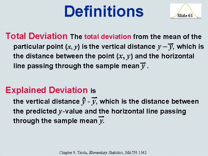
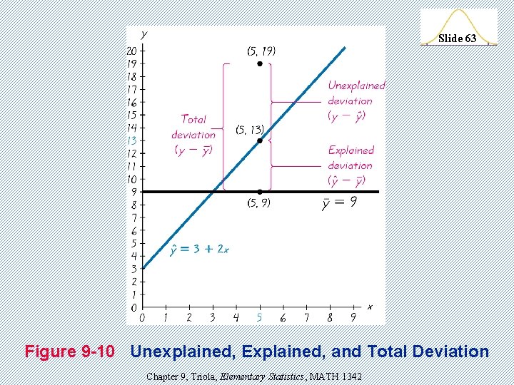
Definitions Slide 61 Total Deviation The total deviation from the mean of the particular point (x, y) is the vertical distance y – y, which is the distance between the point (x, y) and the horizontal line passing through the sample mean y. Explained Deviation is ^ the vertical distance y - y, which is the distance between the predicted y-value and the horizontal line passing through the sample mean y. Chapter 9, Triola, Elementary Statistics, MATH 1342

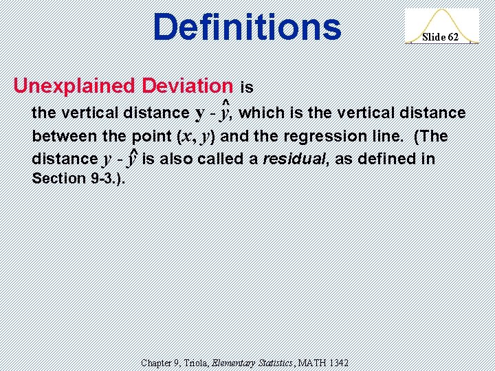
Definitions Unexplained Deviation is Slide 62 the vertical distance y - ^ y, which is the vertical distance between the point (x, y) and the regression line. (The distance y - ^ y is also called a residual, as defined in Section 9 -3. ). Chapter 9, Triola, Elementary Statistics, MATH 1342

Slide 63 Figure 9 -10 Unexplained, Explained, and Total Deviation Chapter 9, Triola, Elementary Statistics, MATH 1342

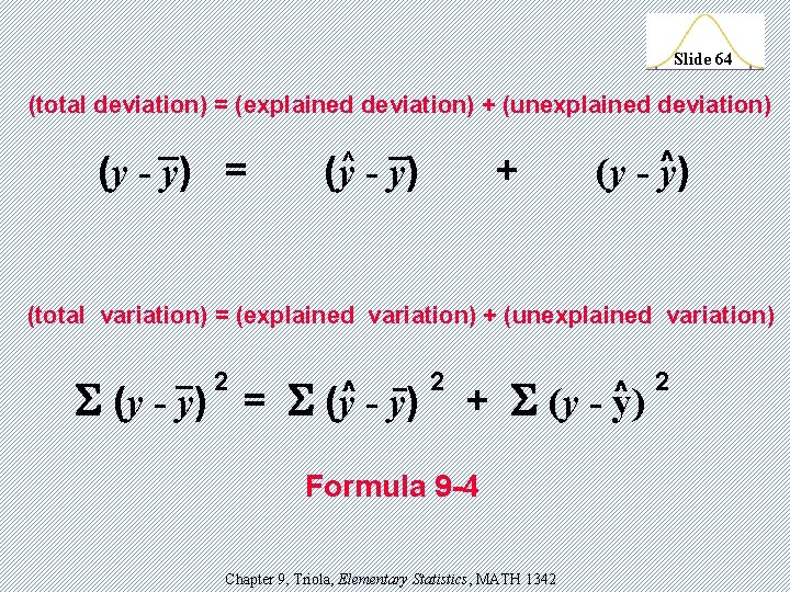
Slide 64 (total deviation) = (explained deviation) + (unexplained deviation) ^ (y - y) = (y - y) + (y - ^ y) (total variation) = (explained variation) + (unexplained variation) (y - y) 2 = (y^ - 2 y) + (y - Formula 9 -4 Chapter 9, Triola, Elementary Statistics, MATH 1342 2 ^ y)

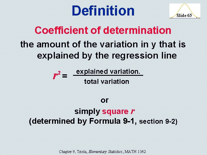
Definition Slide 65 Coefficient of determination the amount of the variation in y that is explained by the regression line r 2 = explained variation. total variation or simply square r (determined by Formula 9 -1, section 9 -2) Chapter 9, Triola, Elementary Statistics, MATH 1342

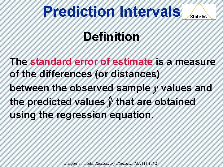
Prediction Intervals Slide 66 Definition The standard error of estimate is a measure of the differences (or distances) between the observed sample y values and the predicted values ^y that are obtained using the regression equation. Chapter 9, Triola, Elementary Statistics, MATH 1342

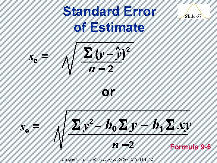
Standard Error of Estimate se = (y Slide 67 2 ^ – y) n – 2 or se = y 2 – b 0 y – b 1 xy n – 2 Chapter 9, Triola, Elementary Statistics, MATH 1342 Formula 9 -5

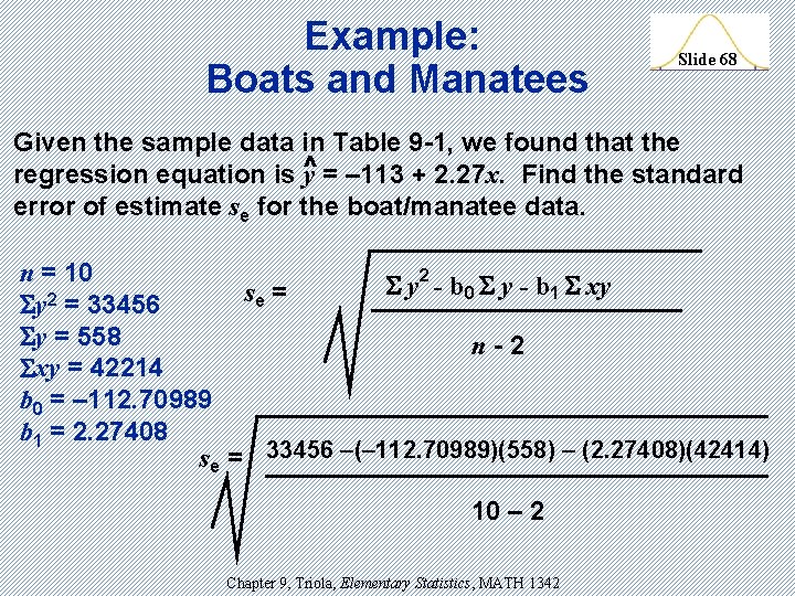
Example: Boats and Manatees Slide 68 Given the sample data in Table 9 -1, we found that the ^ regression equation is y = – 113 + 2. 27 x. Find the standard error of estimate se for the boat/manatee data. 2 n = 10 y - b 1 xy s = 2 e y = 33456 y = 558 n - 2 xy = 42214 b 0 = – 112. 70989 b 1 = 2. 27408 se = 33456 –(– 112. 70989)(558) – (2. 27408)(42414) 10 – 2 Chapter 9, Triola, Elementary Statistics, MATH 1342

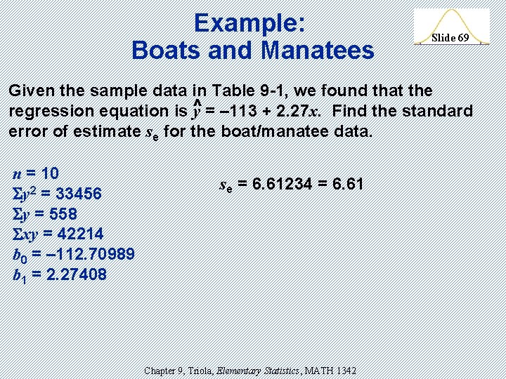
Example: Boats and Manatees Slide 69 Given the sample data in Table 9 -1, we found that the ^ regression equation is y = – 113 + 2. 27 x. Find the standard error of estimate se for the boat/manatee data. n = 10 y 2 = 33456 y = 558 xy = 42214 b 0 = – 112. 70989 b 1 = 2. 27408 se = 6. 61234 = 6. 61 Chapter 9, Triola, Elementary Statistics, MATH 1342

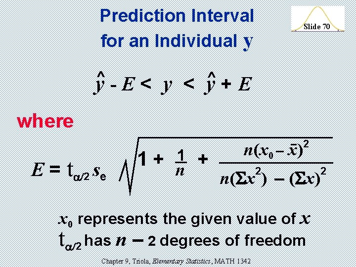
Prediction Interval for an Individual y ^ y - E < y Slide 70 ^ < y + E where E = t 2 se 1 + 1 + n n(x 0 – x) 2 2 n( x ) – ( x) x 0 represents the given value of x t 2 has n – 2 degrees of freedom Chapter 9, Triola, Elementary Statistics, MATH 1342 2

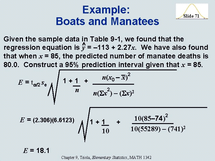
Example: Boats and Manatees Slide 71 Given the sample data in Table 9 -1, we found that the ^ regression equation is y = – 113 + 2. 27 x. We have also found that when x = 85, the predicted number of manatee deaths is 80. 0. Construct a 95% prediction interval given that x = 85. E = t 2 se n(x 0 – x)2 1 + 2 n n( x ) – ( x) 2 E = (2. 306)(6. 6123) 1 + 10 10(85– 74)2 10(55289) – (741)2 E = 18. 1 Chapter 9, Triola, Elementary Statistics, MATH 1342

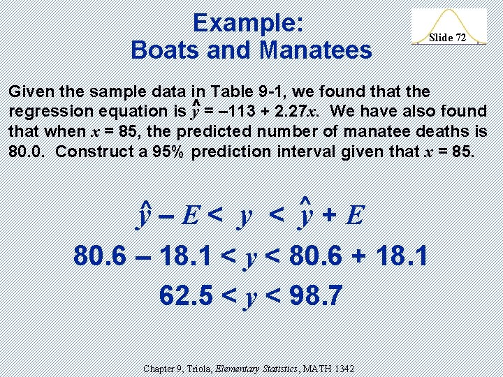
Example: Boats and Manatees Slide 72 Given the sample data in Table 9 -1, we found that the ^ regression equation is y = – 113 + 2. 27 x. We have also found that when x = 85, the predicted number of manatee deaths is 80. 0. Construct a 95% prediction interval given that x = 85. y^ ^ – E < y + E 80. 6 – 18. 1 < y < 80. 6 + 18. 1 62. 5 < y < 98. 7 Chapter 9, Triola, Elementary Statistics, MATH 1342

Slide 73 Section 9 -5 Multiple Regression Created by Erin Hodgess, Houston, Texas

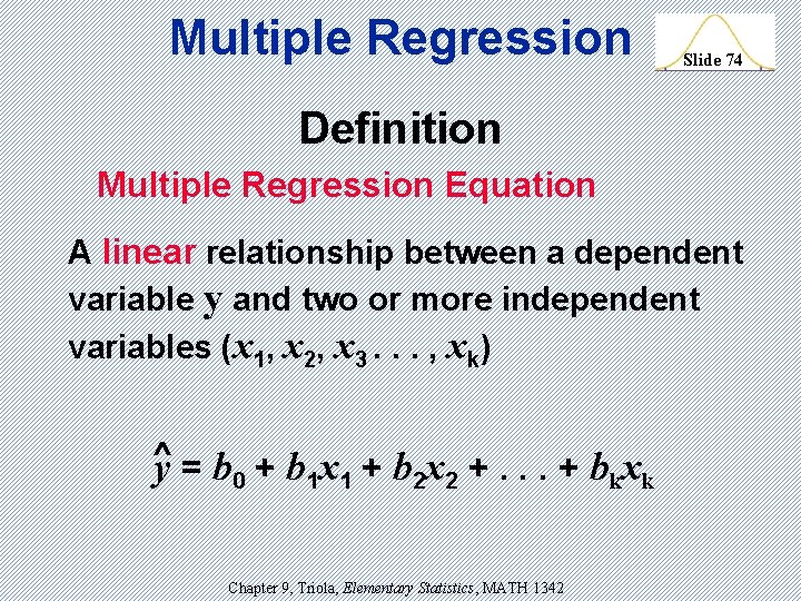
Multiple Regression Slide 74 Definition Multiple Regression Equation A linear relationship between a dependent variable y and two or more independent variables (x 1, x 2, x 3. . . , xk) ^ y = b 0 + b 1 x 1 + b 2 x 2 +. . . + bkxk Chapter 9, Triola, Elementary Statistics, MATH 1342

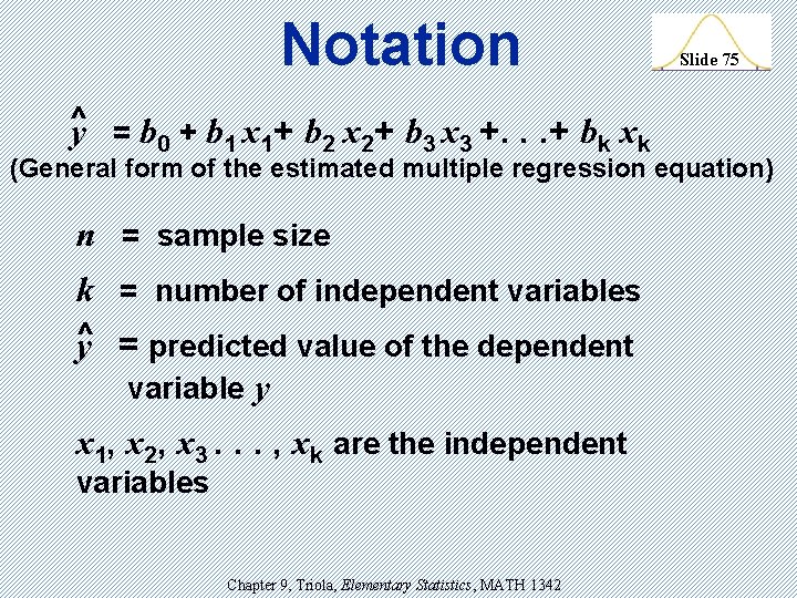
Notation ^y = b 0 + b 1 x 1+ b 2 x 2+ b 3 x 3 +. . . + bk xk Slide 75 (General form of the estimated multiple regression equation) n = sample size k = number of independent variables ^ y = predicted value of the dependent variable y x 1, x 2, x 3. . . , xk are the independent variables Chapter 9, Triola, Elementary Statistics, MATH 1342

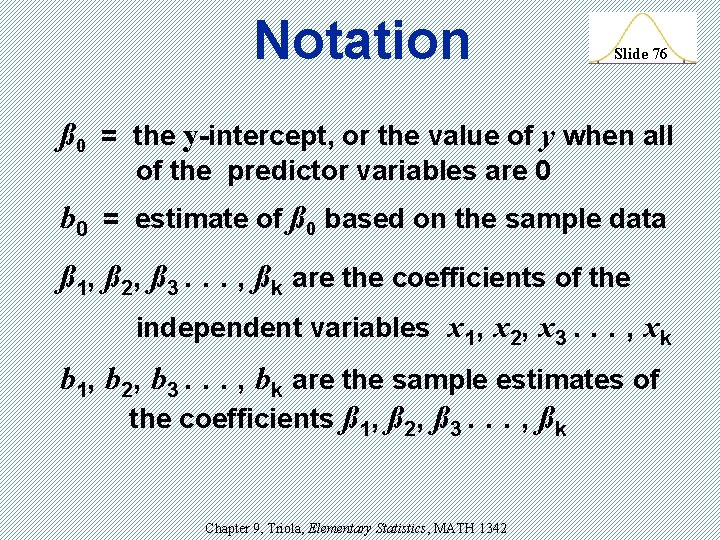
Notation Slide 76 ß 0 = the y-intercept, or the value of y when all of the predictor variables are 0 b 0 = estimate of ß 0 based on the sample data ß 1, ß 2, ß 3. . . , ßk are the coefficients of the independent variables x 1, x 2, x 3. . . , xk b 1, b 2, b 3. . . , bk are the sample estimates of the coefficients ß 1, ß 2, ß 3. . . , ßk Chapter 9, Triola, Elementary Statistics, MATH 1342

Assumption Slide 77 Use a statistical software package such as v STATDISK v Minitab v Excel Chapter 9, Triola, Elementary Statistics, MATH 1342

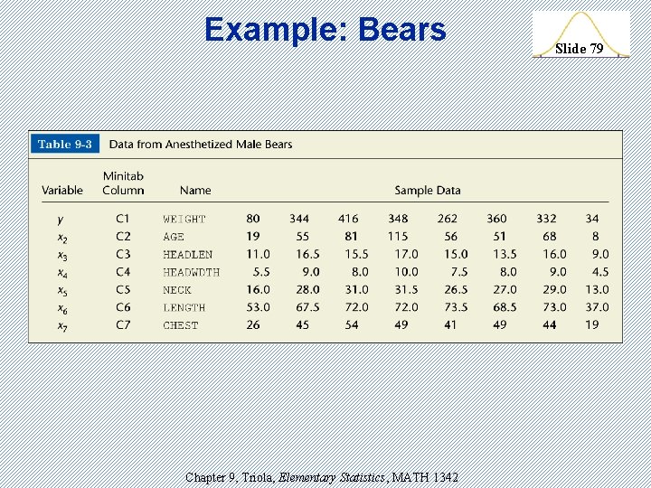
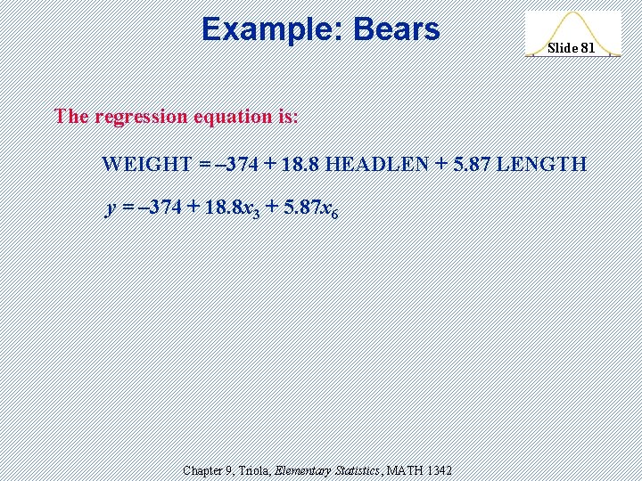
Example: Bears Slide 78 For reasons of safety, a study of bears involved the collection of various measurements that were taken after the bears were anesthetized. Using the data in Table 9 -3, find the multiple regression equation in which the dependent variable is weight and the independent variables are head length and total overall length. Chapter 9, Triola, Elementary Statistics, MATH 1342

Example: Bears Chapter 9, Triola, Elementary Statistics, MATH 1342 Slide 79

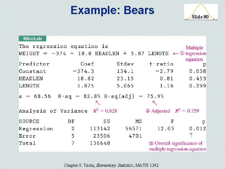
Example: Bears Chapter 9, Triola, Elementary Statistics, MATH 1342 Slide 80

Example: Bears Slide 81 The regression equation is: WEIGHT = – 374 + 18. 8 HEADLEN + 5. 87 LENGTH y = – 374 + 18. 8 x 3 + 5. 87 x 6 Chapter 9, Triola, Elementary Statistics, MATH 1342

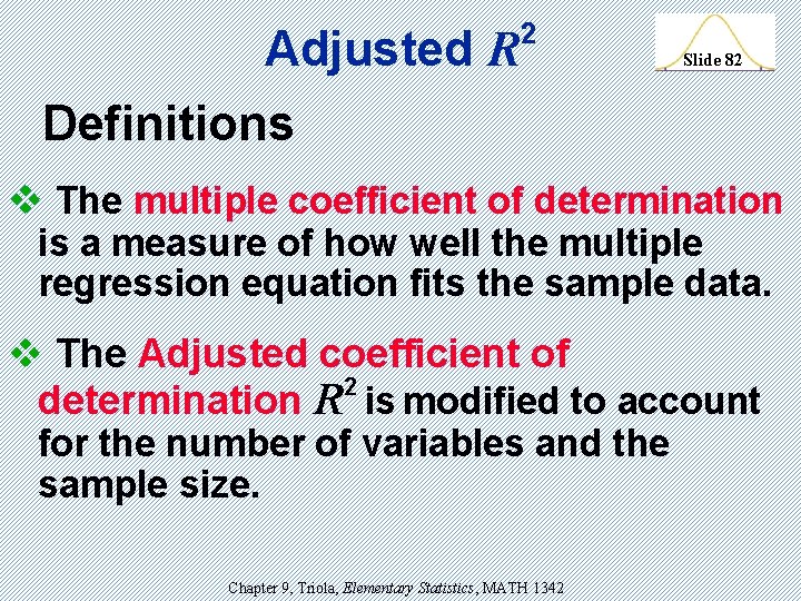
Adjusted R 2 Slide 82 Definitions v The multiple coefficient of determination is a measure of how well the multiple regression equation fits the sample data. v The Adjusted coefficient of 2 determination R is modified to account for the number of variables and the sample size. Chapter 9, Triola, Elementary Statistics, MATH 1342

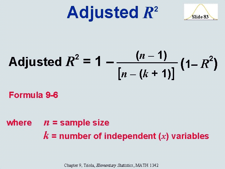
Adjusted R 2 Adjusted R = 1 – 2 (n – 1) [n – (k + 1)] Slide 83 2 (1– R ) Formula 9 -6 where n = sample size k = number of independent (x) variables Chapter 9, Triola, Elementary Statistics, MATH 1342

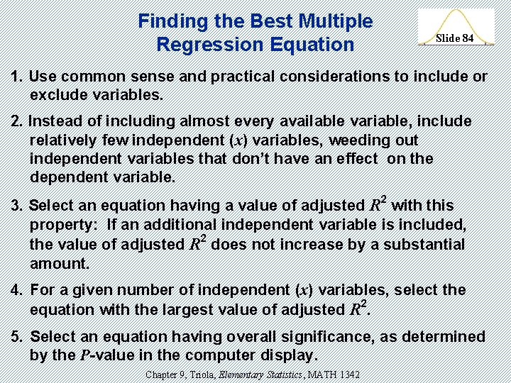
Finding the Best Multiple Regression Equation Slide 84 1. Use common sense and practical considerations to include or exclude variables. 2. Instead of including almost every available variable, include relatively few independent (x) variables, weeding out independent variables that don’t have an effect on the dependent variable. 3. Select an equation having a value of adjusted R 2 with this property: If an additional independent variable is included, the value of adjusted R 2 does not increase by a substantial amount. 4. For a given number of independent (x) variables, select the equation with the largest value of adjusted R 2. 5. Select an equation having overall significance, as determined by the P-value in the computer display. Chapter 9, Triola, Elementary Statistics, MATH 1342

Slide 85 Section 9 -6 Modeling Created by Erin Hodgess, Houston, Texas

Definition Slide 86 Mathematical Model A mathematical model is a mathematical function that ‘fits’ or describes real-world data. Chapter 9, Triola, Elementary Statistics, MATH 1342

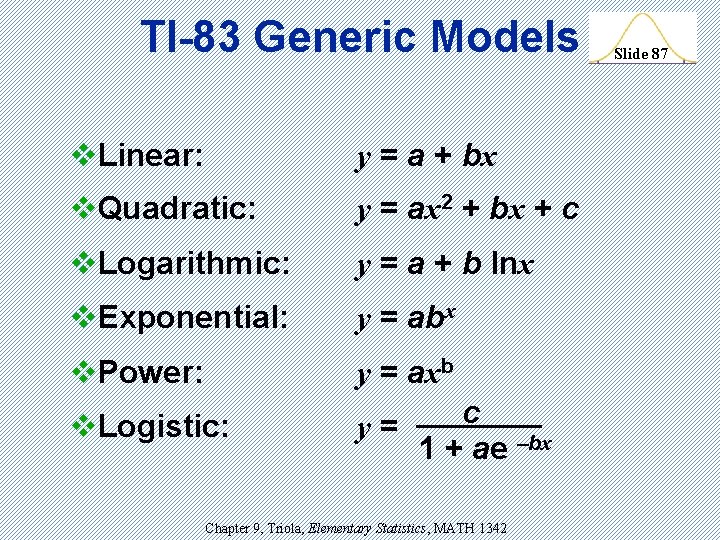
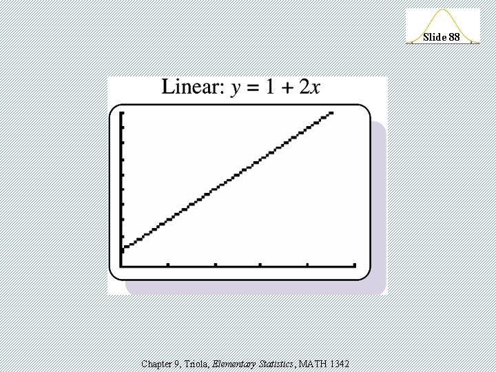
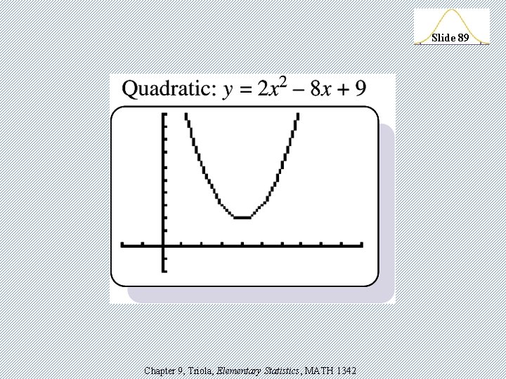
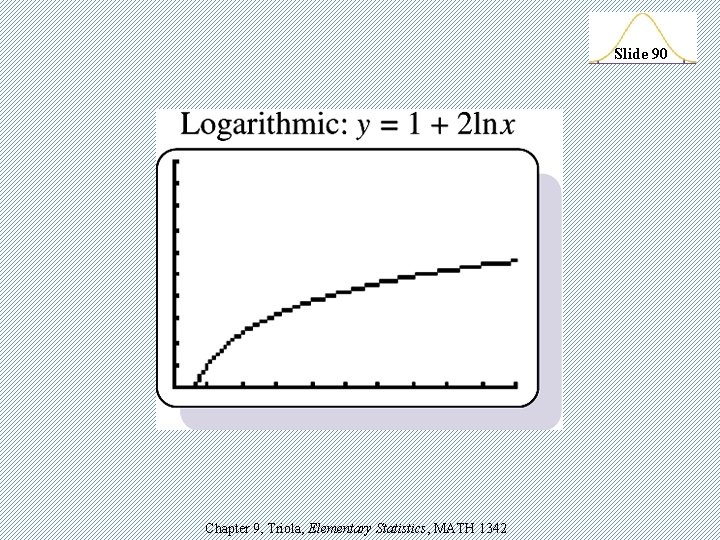
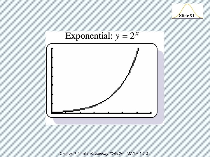
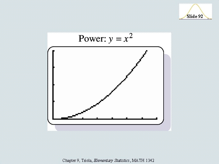
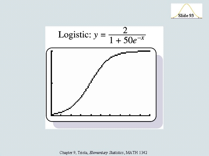
TI-83 Generic Models v. Linear: y = a + bx v. Quadratic: y = ax 2 + bx + c v. Logarithmic: y = a + b lnx v. Exponential: y = abx v. Power: y = axb v. Logistic: c y = 1 + ae –bx Chapter 9, Triola, Elementary Statistics, MATH 1342 Slide 87

Slide 88 Chapter 9, Triola, Elementary Statistics, MATH 1342

Slide 89 Chapter 9, Triola, Elementary Statistics, MATH 1342

Slide 90 Chapter 9, Triola, Elementary Statistics, MATH 1342

Slide 91 Chapter 9, Triola, Elementary Statistics, MATH 1342

Slide 92 Chapter 9, Triola, Elementary Statistics, MATH 1342

Slide 93 Chapter 9, Triola, Elementary Statistics, MATH 1342

Development of a Good Mathematics Model Slide 94 v Look for a Pattern in the Graph: Examine the graph of the plotted points and compare the basic pattern to the known generic graphs. v Find and Compare Values of R 2: Select functions that result in larger values of R 2, because such larger values correspond to functions that better fit the observed points. v Think: Use common sense. Don’t use a model that lead to predicted values known to be totally unrealistic. Chapter 9, Triola, Elementary Statistics, MATH 1342