Chapter 9 Queuing Models 1 9 1 Introduction

Chapter 9 Queuing Models 1

9. 1 Introduction • Queuing is the study of waiting lines, or queues. • The objective of queuing analysis is to design systems that enable organizations to perform optimally according to some criterion. • Possible Criteria – Maximum Profits. – Desired Service Level. 2

9. 1 Introduction • Analyzing queuing systems requires a clear understanding of the appropriate service measurement. • Possible service measurements – Average time a customer spends in line. – Average length of the waiting line. – The probability that an arriving customer must wait for service. 3

9. 2 Elements of the Queuing Process • A queuing system consists of three basic components: – Arrivals: Customers arrive according to some arrival pattern. – Waiting in a queue: Arriving customers may have to wait in one or more queues for service. – Service: Customers receive service and leave the system. 4

The Arrival Process • There are two possible types of arrival processes – Deterministic arrival process. – Random arrival process. • The random process is more common in businesses. 5

The Arrival Process • Under three conditions the arrivals can be modeled as a Poisson process – Orderliness : one customer, at most, will arrive during any time interval. – Stationarity : for a given time frame, the probability of arrivals within a certain time interval is the same for all time intervals of equal length. – Independence : the arrival of one customer has no influence on the arrival of another. 6

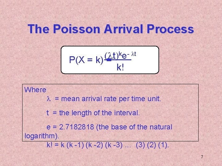
The Poisson Arrival Process ke- lt (lt) P(X = k) = k! Where l = mean arrival rate per time unit. t = the length of the interval. e = 2. 7182818 (the base of the natural logarithm). k! = k (k -1) (k -2) (k -3) … (3) (2) (1). 7

HANK’s HARDWARE – Arrival Process • Customers arrive at Hank’s Hardware according to a Poisson distribution. • Between 8: 00 and 9: 00 A. M. an average of 6 customers arrive at the store. • What is the probability that k customers will arrive between 8: 00 and 8: 30 in the morning (k = 0, 1, 2, …)? 8

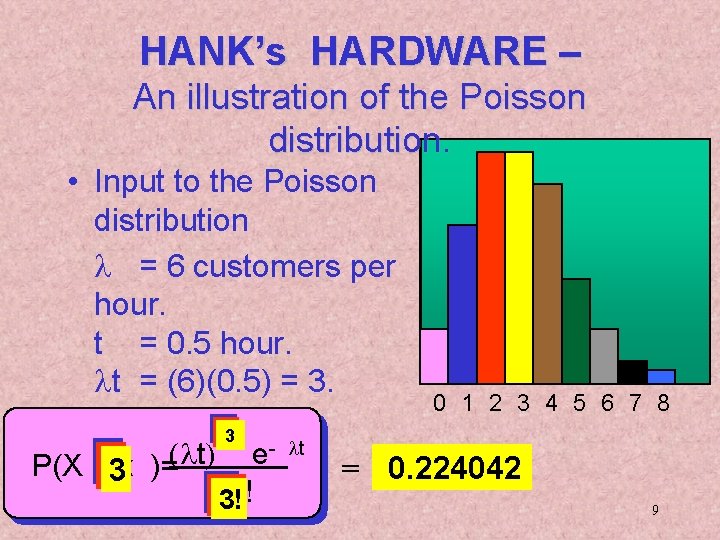
HANK’s HARDWARE – An illustration of the Poisson distribution. • Input to the Poisson distribution l = 6 customers per hour. t = 0. 5 hour. lt = (6)(0. 5) = 3. (lt) e P(X =0123 k )= k! 1! 0! 2! 3! 10 k 23 lt 0 1 2 3 4 5 6 7 8 = 0. 224042 0. 149361 0. 049787 0. 224042 9

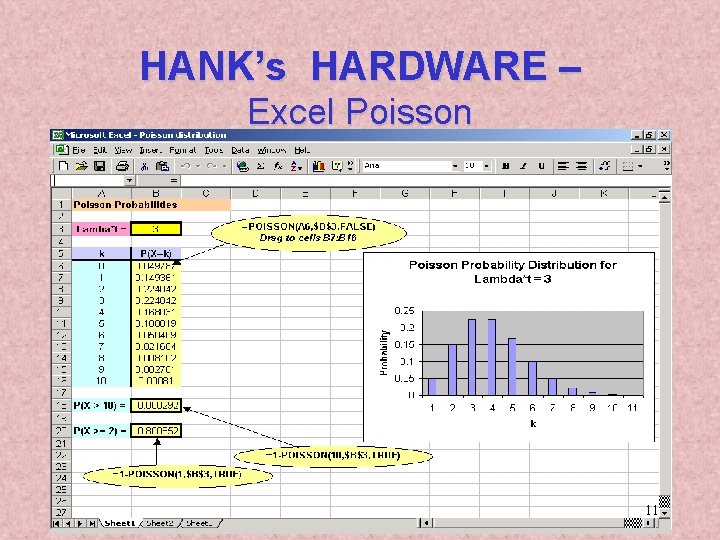
HANK’s HARDWARE – Using Excel for the Poisson probabilities • Solution – We can use the POISSON function in Excel to determine Poisson probabilities. – Point probability: P(X = k) = ? • Use Poisson(k, lt, FALSE) • Example: P(X = 0; lt = 3) = POISSON(0, 1. 5, FALSE) – Cumulative probability: P(X£k) = ? • Example: P(X£ 3; lt = 3) = Poisson(3, 1. 5, TRUE) 10

HANK’s HARDWARE – Excel Poisson 11

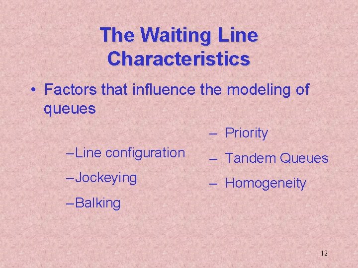
The Waiting Line Characteristics • Factors that influence the modeling of queues – Priority – Line configuration – Tandem Queues – Jockeying – Homogeneity – Balking 12

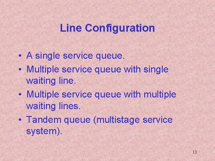
Line Configuration • A single service queue. • Multiple service queue with single waiting line. • Multiple service queue with multiple waiting lines. • Tandem queue (multistage service system). 13

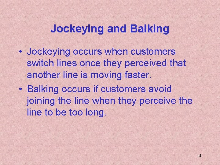
Jockeying and Balking • Jockeying occurs when customers switch lines once they perceived that another line is moving faster. • Balking occurs if customers avoid joining the line when they perceive the line to be too long. 14

Priority Rules • These rules select the next customer for service. • There are several commonly used rules: – First come first served (FCFS). – Last come first served (LCFS). – Estimated service time. – Random selection of customers for service. 15

Tandem Queues • These are multi-server systems. • A customer needs to visit several service stations (usually in a distinct order) to complete the service process. • Examples – Patients in an emergency room. – Passengers prepare for the next flight. 16

Homogeneity • A homogeneous customer population is one in which customers require essentially the same type of service. • A non-homogeneous customer population is one in which customers can be categorized according to: – Different arrival patterns – Different service treatments. 17

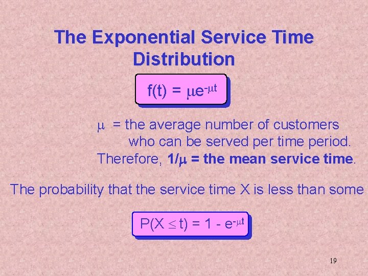
The Service Process • In most business situations, service time varies widely among customers. • When service time varies, it is treated as a random variable. • The exponential probability distribution is used sometimes to model customer service time. 18

The Exponential Service Time Distribution f(t) = me-mt m = the average number of customers who can be served per time period. Therefore, 1/m = the mean service time. The probability that the service time X is less than some P(X £ t) = 1 - e-mt 19

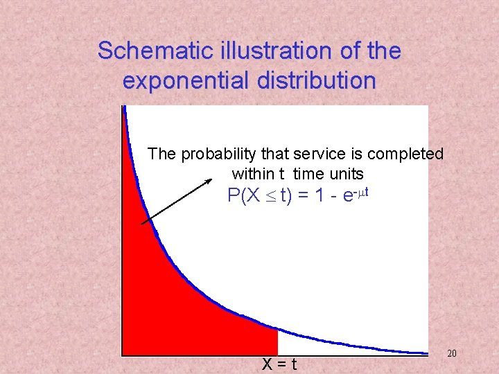
Schematic illustration of the exponential distribution The probability that service is completed within t time units P(X £ t) = 1 - e-mt X=t 20

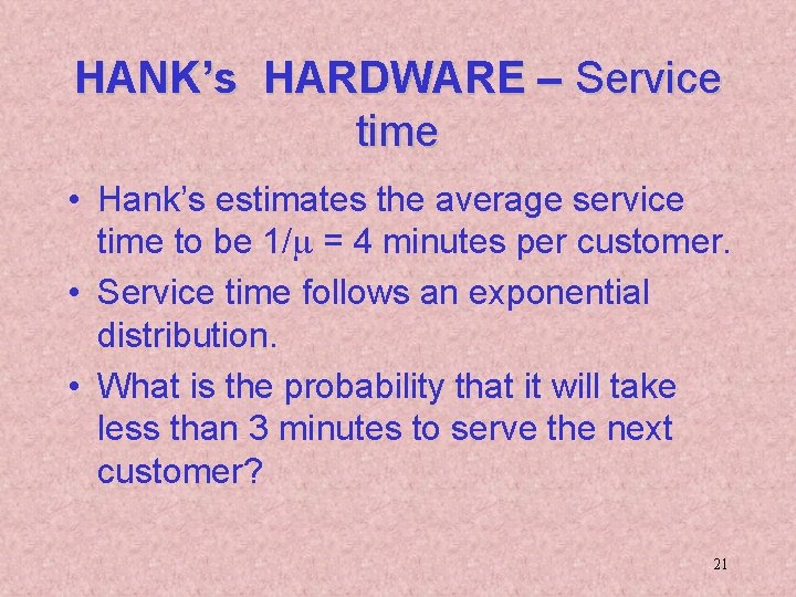
HANK’s HARDWARE – Service time • Hank’s estimates the average service time to be 1/m = 4 minutes per customer. • Service time follows an exponential distribution. • What is the probability that it will take less than 3 minutes to serve the next customer? 21

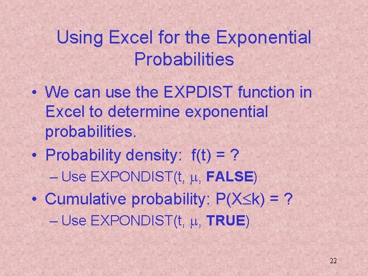
Using Excel for the Exponential Probabilities • We can use the EXPDIST function in Excel to determine exponential probabilities. • Probability density: f(t) = ? – Use EXPONDIST(t, m, FALSE) • Cumulative probability: P(X£k) = ? – Use EXPONDIST(t, m, TRUE) 22

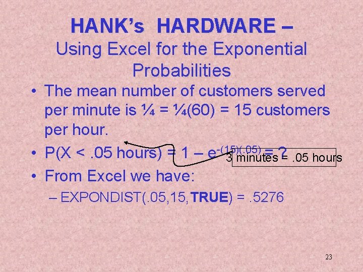
HANK’s HARDWARE – Using Excel for the Exponential Probabilities • The mean number of customers served per minute is ¼ = ¼(60) = 15 customers per hour. • P(X <. 05 hours) = 1 – e-(15)(. 05) = ? =. 05 hours 3 minutes • From Excel we have: – EXPONDIST(. 05, 15, TRUE) =. 5276 23

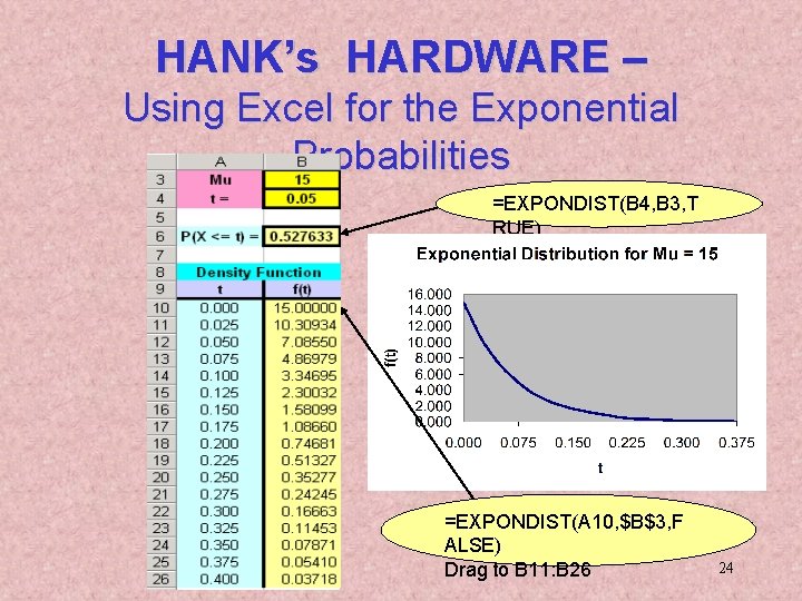
HANK’s HARDWARE – Using Excel for the Exponential Probabilities =EXPONDIST(B 4, B 3, T RUE) =EXPONDIST(A 10, $B$3, F ALSE) Drag to B 11: B 26 24

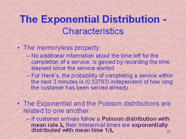
The Exponential Distribution Characteristics • The memoryless property. – No additional information about the time left for the completion of a service, is gained by recording the time elapsed since the service started. – For Hank’s, the probability of completing a service within the next 3 minutes is (0. 52763) independent of how long the customer has been served already. • The Exponential and the Poisson distributions are related to one another. – If customer arrivals follow a Poisson distribution with mean rate l, their interarrival times are exponentially distributed with mean time 1/l. 25

9. 3 Performance Measures of Queuing System • Performance can be measured by focusing on: – Customers in queue. – Customers in the system. • Performance is measured for a system in steady state. 26

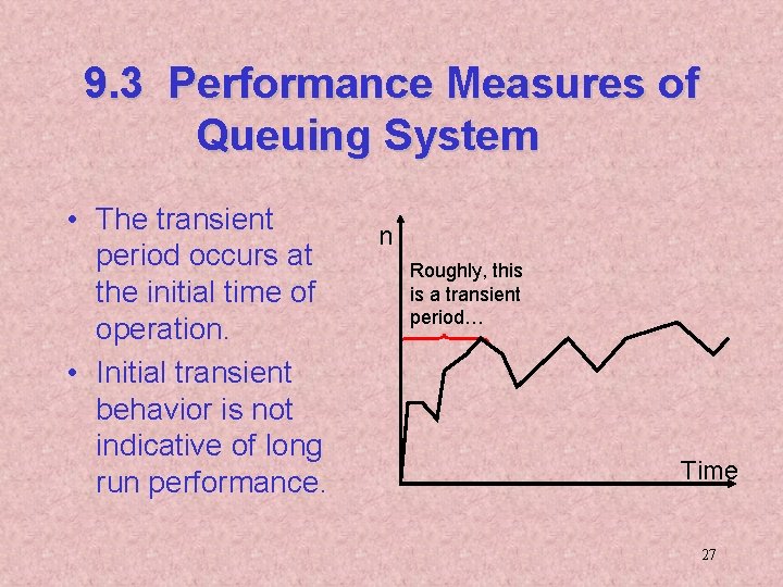
9. 3 Performance Measures of Queuing System • The transient period occurs at the initial time of operation. • Initial transient behavior is not indicative of long run performance. n Roughly, this is a transient period… Time 27

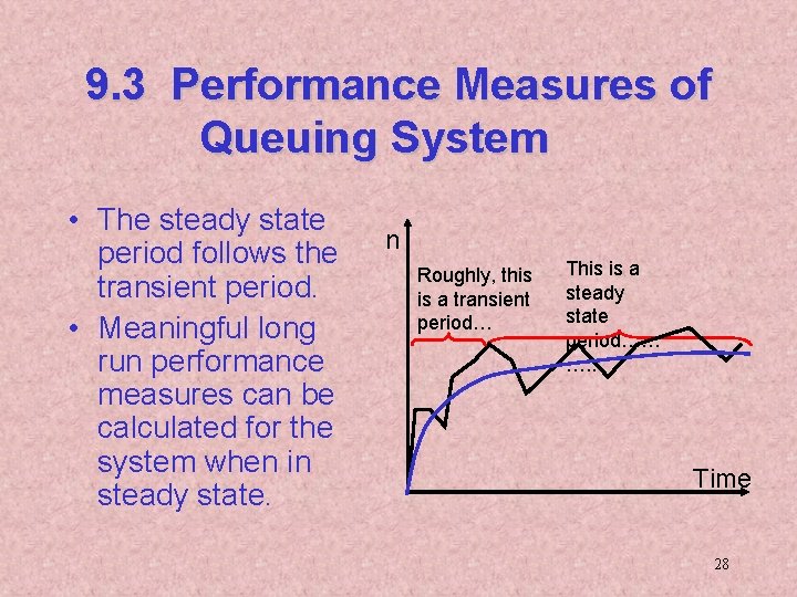
9. 3 Performance Measures of Queuing System • The steady state period follows the transient period. • Meaningful long run performance measures can be calculated for the system when in steady state. n Roughly, this is a transient period… This is a steady state period…… …. . Time 28

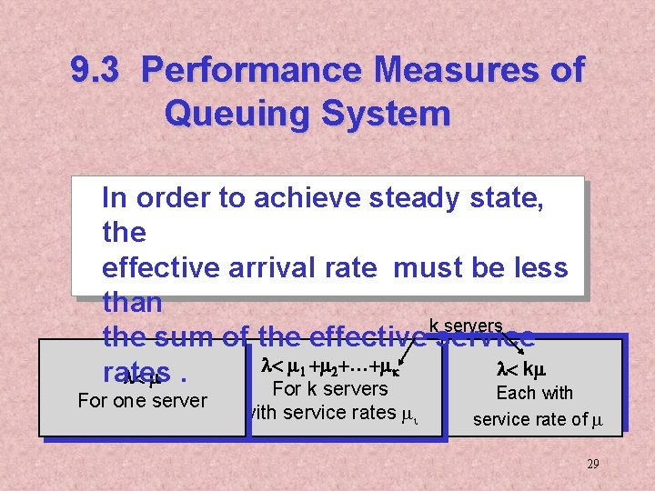
9. 3 Performance Measures of Queuing System In order to achieve steady state, the effective arrival rate must be less than k servers the sum of the effective service l< m 1 +m 2+…+mk l< km rates l< m. For k servers For one server with service rates mi Each with service rate of m 29

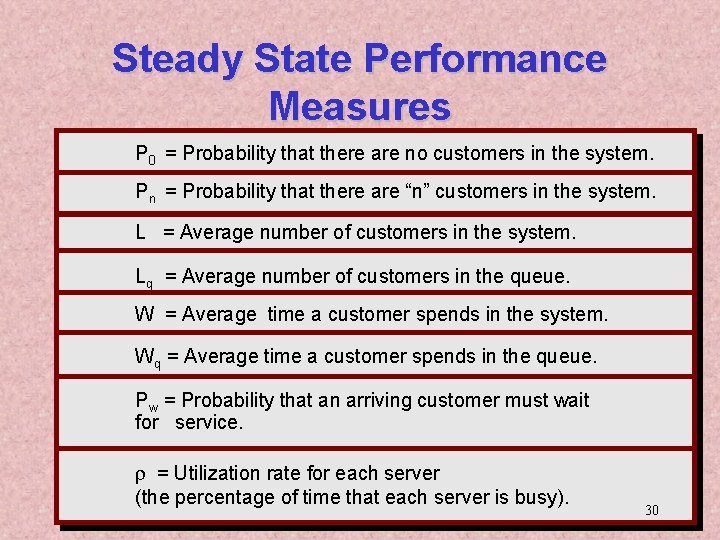
Steady State Performance Measures P 0 = Probability that there are no customers in the system. Pn = Probability that there are “n” customers in the system. L = Average number of customers in the system. Lq = Average number of customers in the queue. W = Average time a customer spends in the system. Wq = Average time a customer spends in the queue. Pw = Probability that an arriving customer must wait for service. r = Utilization rate for each server (the percentage of time that each server is busy). 30

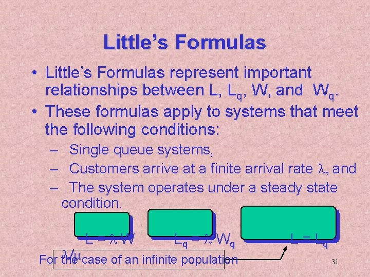
Little’s Formulas • Little’s Formulas represent important relationships between L, Lq, W, and Wq. • These formulas apply to systems that meet the following conditions: – Single queue systems, – Customers arrive at a finite arrival rate l, and – The system operates under a steady state condition. L = l W L q = l Wq l/mcase of an infinite population For the L = Lq + 31

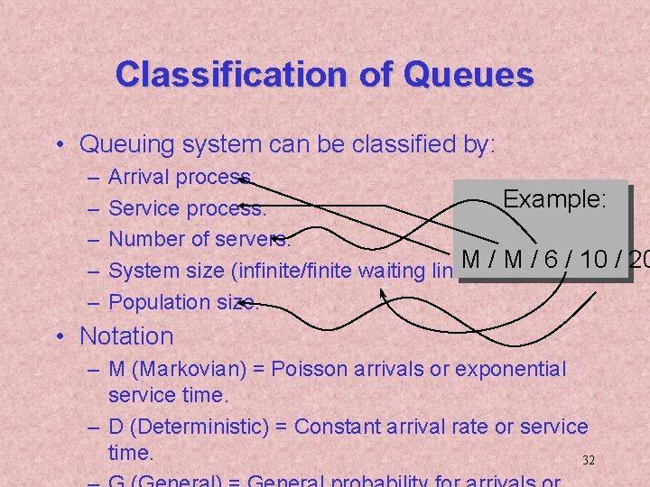
Classification of Queues • Queuing system can be classified by: – – – Arrival process. Example: Service process. Number of servers. M / 6 / 10 / 20 System size (infinite/finite waiting line). Population size. • Notation – M (Markovian) = Poisson arrivals or exponential service time. – D (Deterministic) = Constant arrival rate or service time. 32

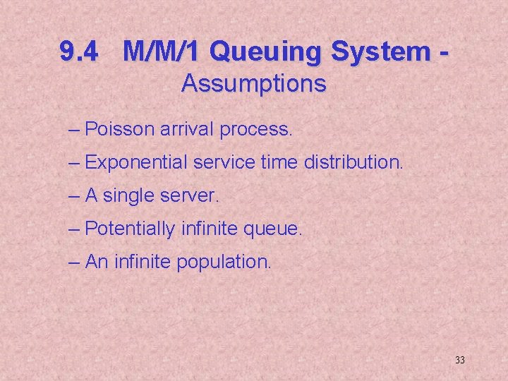
9. 4 M/M/1 Queuing System Assumptions – Poisson arrival process. – Exponential service time distribution. – A single server. – Potentially infinite queue. – An infinite population. 33

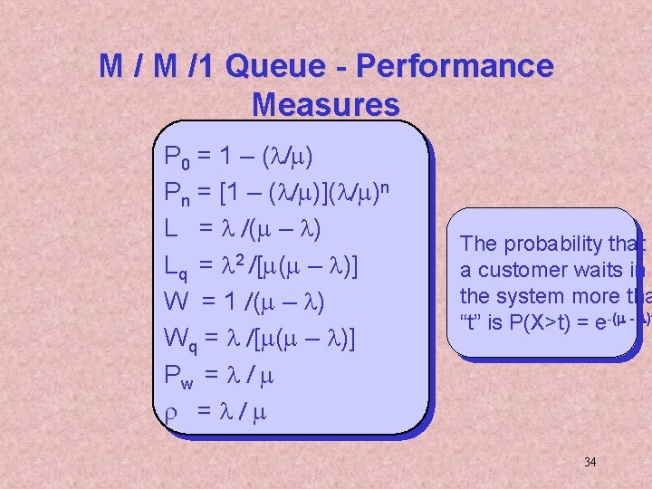
M / M /1 Queue - Performance Measures P 0 = 1 – (l/m) Pn = [1 – (l/m)](l/m)n L = l /(m – l) Lq = l 2 /[m(m – l)] W = 1 /(m – l) Wq = l /[m(m – l)] Pw = l / m r = l / m The probability that a customer waits in the system more tha “t” is P(X>t) = e-(m - l)t 34

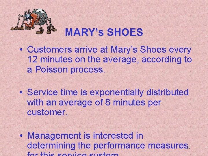
MARY’s SHOES • Customers arrive at Mary’s Shoes every 12 minutes on the average, according to a Poisson process. • Service time is exponentially distributed with an average of 8 minutes per customer. • Management is interested in determining the performance measures 35

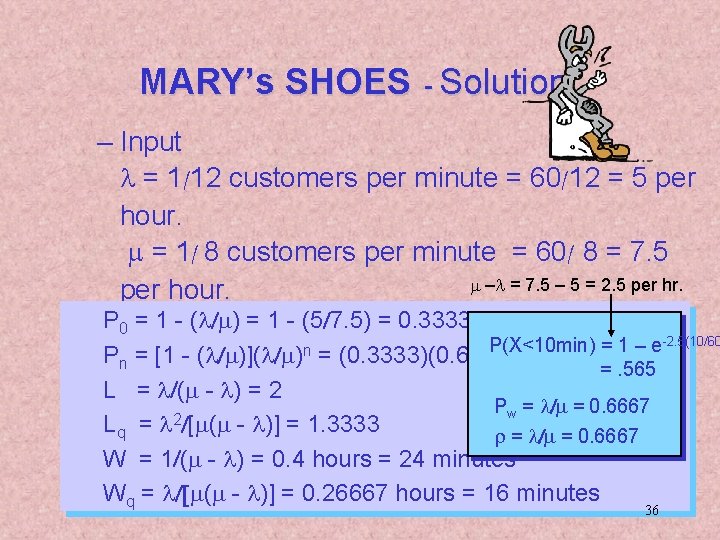
MARY’s SHOES - Solution – Input l = 1/12 customers per minute = 60/12 = 5 per hour. m = 1/ 8 customers per minute = 60/ 8 = 7. 5 m –l = 7. 5 – 5 = 2. 5 per hr. per hour. P 0 = 1 - (l/m) = 1 - (5/7. 5) = 0. 3333 –PPerformance Calculations P(X<10 min) = 1 – e-2. 5(10/60 n n n = [1 - (l/m)](l/m) = (0. 3333)(0. 6667) =. 565 L = l/(m - l) = 2 Pw = l/m = 0. 6667 2 Lq = l /[m(m - l)] = 1. 3333 r = l/m = 0. 6667 W = 1/(m - l) = 0. 4 hours = 24 minutes Wq = l/[m(m - l)] = 0. 26667 hours = 16 minutes 36

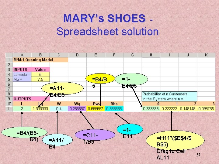
MARY’s SHOES Spreadsheet solution =A 11 B 4/B 5 =B 4/(B 5 B 4) =A 11/ B 4 =B 4/B 5 =C 111/B 5 =1 B 4/B 5 =1 E 11 =H 11*($B$4/$ B$5) Drag to Cell AL 11 37

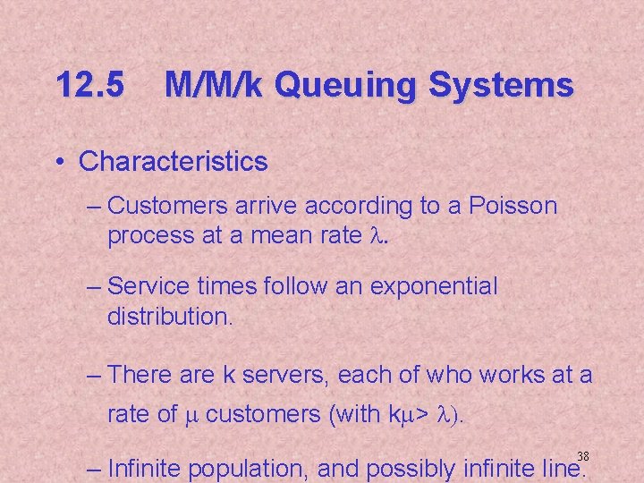
12. 5 M/M/k Queuing Systems • Characteristics – Customers arrive according to a Poisson process at a mean rate l. – Service times follow an exponential distribution. – There are k servers, each of who works at a rate of m customers (with km> l). 38 – Infinite population, and possibly infinite line.

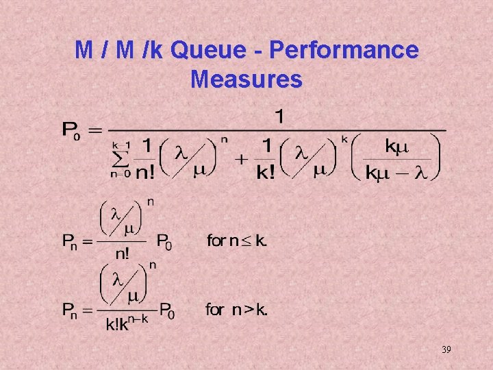
M / M /k Queue - Performance Measures 39

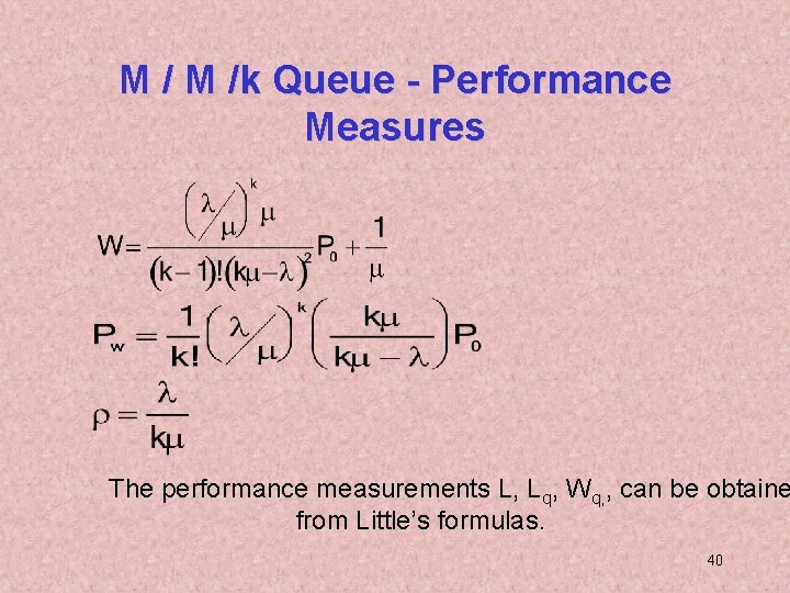
M / M /k Queue - Performance Measures The performance measurements L, Lq, Wq, , can be obtaine from Little’s formulas. 40

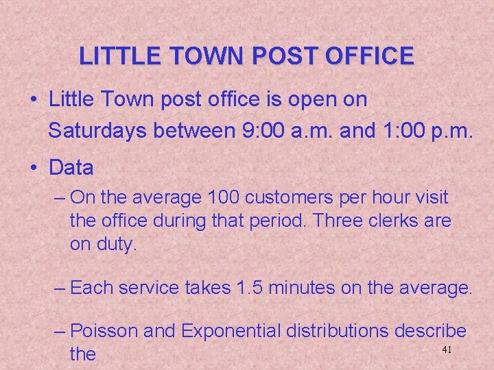
LITTLE TOWN POST OFFICE • Little Town post office is open on Saturdays between 9: 00 a. m. and 1: 00 p. m. • Data – On the average 100 customers per hour visit the office during that period. Three clerks are on duty. – Each service takes 1. 5 minutes on the average. – Poisson and Exponential distributions describe 41 the

LITTLE TOWN POST OFFICE • The Postmaster needs to know the relevant service measures in order to: – Evaluate the current service level. – Study the effects of reducing the staff by one clerk. 42

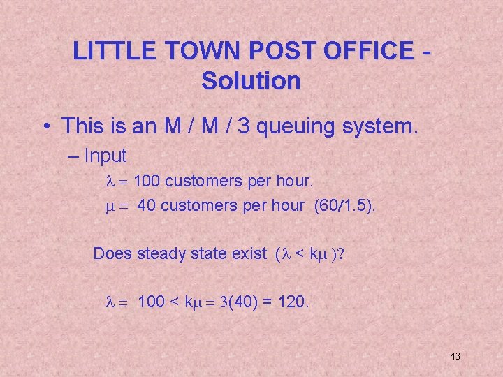
LITTLE TOWN POST OFFICE Solution • This is an M / 3 queuing system. – Input l = 100 customers per hour. m = 40 customers per hour (60/1. 5). Does steady state exist (l < km )? l = 100 < km = 3(40) = 120. 43

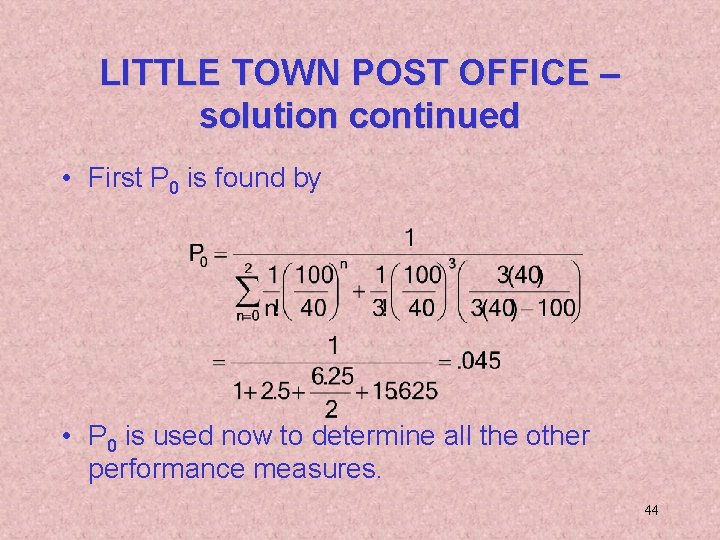
LITTLE TOWN POST OFFICE – solution continued • First P 0 is found by • P 0 is used now to determine all the other performance measures. 44

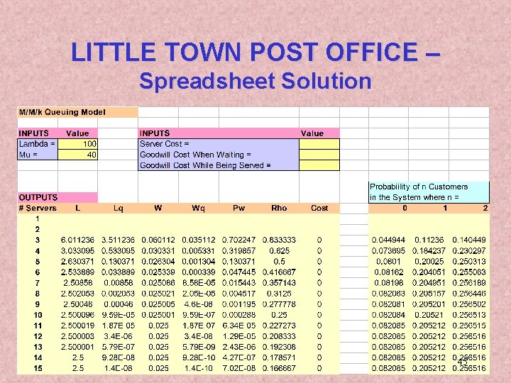
LITTLE TOWN POST OFFICE – Spreadsheet Solution 45

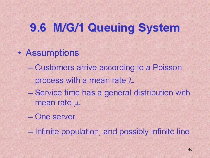
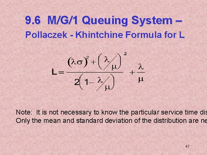
9. 6 M/G/1 Queuing System • Assumptions – Customers arrive according to a Poisson process with a mean rate l. – Service time has a general distribution with mean rate m. – One server. – Infinite population, and possibly infinite line. 46

9. 6 M/G/1 Queuing System – Pollaczek - Khintchine Formula for L Note: It is not necessary to know the particular service time dis Only the mean and standard deviation of the distribution are ne 47

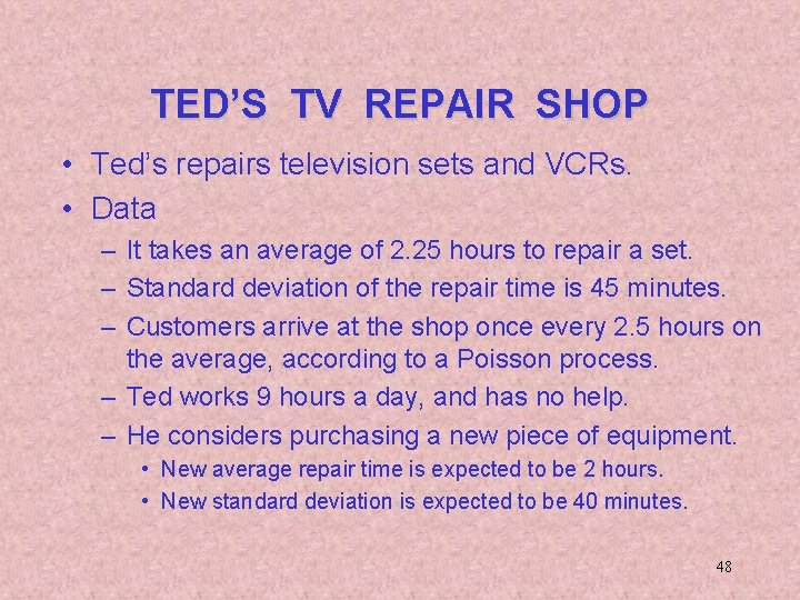
TED’S TV REPAIR SHOP • Ted’s repairs television sets and VCRs. • Data – It takes an average of 2. 25 hours to repair a set. – Standard deviation of the repair time is 45 minutes. – Customers arrive at the shop once every 2. 5 hours on the average, according to a Poisson process. – Ted works 9 hours a day, and has no help. – He considers purchasing a new piece of equipment. • New average repair time is expected to be 2 hours. • New standard deviation is expected to be 40 minutes. 48

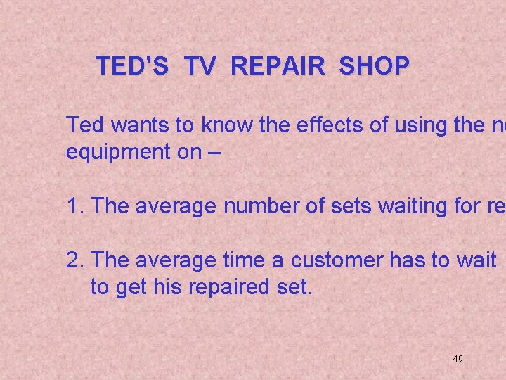
TED’S TV REPAIR SHOP Ted wants to know the effects of using the ne equipment on – 1. The average number of sets waiting for re 2. The average time a customer has to wait to get his repaired set. 49

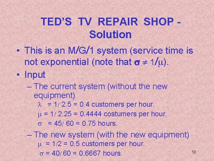
TED’S TV REPAIR SHOP Solution • This is an M/G/1 system (service time is not exponential (note that s ¹ 1/m). • Input – The current system (without the new equipment) l = 1/ 2. 5 = 0. 4 customers per hour. m = 1/ 2. 25 = 0. 4444 costumers per hour. s = 45/ 60 = 0. 75 hours. – The new system (with the new equipment) m = 1/2 = 0. 5 customers per hour. s = 40/ 60 = 0. 6667 hours. 50

9. 7 M / k / F Queuing System • Many times queuing systems have designs that limit their line size. • When the potential queue is large, an infinite queue model gives accurate results, even though the queue might be limited. • When the potential queue is small, the limited line must be accounted for in the 51

Characteristics of M/M/k/F Queuing System • Poisson arrival process at mean rate l. • k servers, each having an exponential service time with mean rate m. • Maximum number of customers that can be present in the system at any one time is “F”. 52

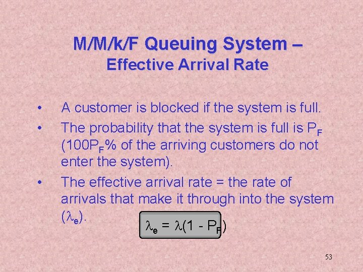
M/M/k/F Queuing System – Effective Arrival Rate • • • A customer is blocked if the system is full. The probability that the system is full is PF (100 PF% of the arriving customers do not enter the system). The effective arrival rate = the rate of arrivals that make it through into the system (le). le = l(1 - PF) 53

RYAN ROOFING COMPANY • Ryan gets most of its business from customers who call and order service. – When a telephone line is available but the secretary is busy serving a customer, a new calling customer is willing to wait until the secretary becomes available. – When all the lines are busy, a new calling customer gets a busy signal and calls a competitor. 54

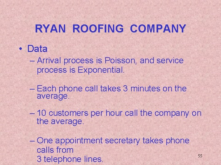
RYAN ROOFING COMPANY • Data – Arrival process is Poisson, and service process is Exponential. – Each phone call takes 3 minutes on the average. – 10 customers per hour call the company on the average. – One appointment secretary takes phone calls from 3 telephone lines. 55

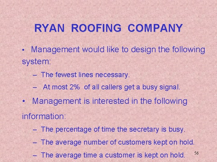
RYAN ROOFING COMPANY • Management would like to design the following system: – The fewest lines necessary. – At most 2% of all callers get a busy signal. • Management is interested in the following information: – The percentage of time the secretary is busy. – The average number of customers kept on hold. – The average time a customer is kept on hold. 56

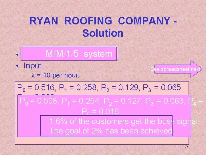
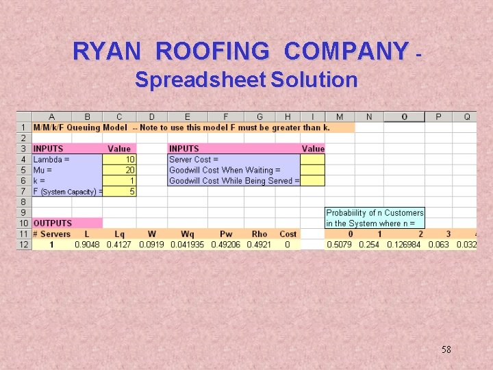
RYAN ROOFING COMPANY Solution M/M/1/4 system • This is. M/M/1/5 an M/M/1/system 3 system • Input l = 10 per hour. See spreadsheet next = 20 per (1/3 per P 0 m = 0. 516, P 1 hour = 0. 258, P 2 minute). = 0. 129, P 3 = 0. 065, • P 4 Excel spreadsheet gives: = 0. 032 P 0 = 0. 508, P 1 = 0. 254, P 2 = 0. 127, P 3 = 0. 063, P 4 = 0 P 0 = 0. 533, P 1 = 0. 133, P 3 = 0. 06 P 5 = 0. 016 3. 2% the customers getsignal. the busy signal 6. 7% of 1. 6% theofcustomers get a busy of the customers get busy signal Still above the goal of achieved. 2% The goal of 2% has been This is above the goal of 2%. 57

RYAN ROOFING COMPANY Spreadsheet Solution 58

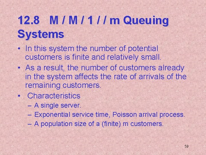
12. 8 M / 1 / / m Queuing Systems • In this system the number of potential customers is finite and relatively small. • As a result, the number of customers already in the system affects the rate of arrivals of the remaining customers. • Characteristics – A single server. – Exponential service time, Poisson arrival process. – A population size of a (finite) m customers. 59

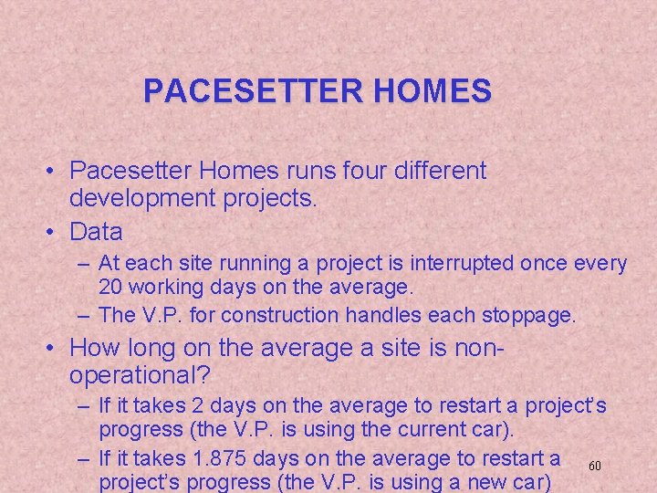
PACESETTER HOMES • Pacesetter Homes runs four different development projects. • Data – At each site running a project is interrupted once every 20 working days on the average. – The V. P. for construction handles each stoppage. • How long on the average a site is nonoperational? – If it takes 2 days on the average to restart a project’s progress (the V. P. is using the current car). – If it takes 1. 875 days on the average to restart a 60 project’s progress (the V. P. is using a new car)

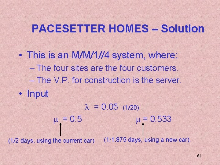
PACESETTER HOMES – Solution • This is an M/M/1//4 system, where: – The four sites are the four customers. – The V. P. for construction is the server. • Input l = 0. 05 m = 0. 5 (1/2 days, using the current car) (1/20) m = 0. 533 (1/1. 875 days, using a new car). 61

PACESETTER HOMES – Solution continued Summary of results 62

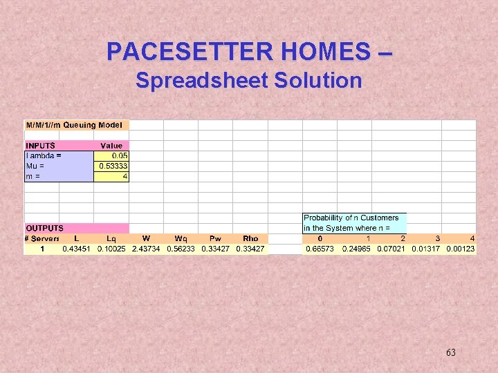
PACESETTER HOMES – Spreadsheet Solution 63

9. 9 Economic Analysis of Queuing Systems • The performance measures previously developed are used next to determine a minimal cost queuing system. • The procedure requires estimated costs such as: – Hourly cost per server. – Customer goodwill cost while waiting in line. – Customer goodwill cost while being served. 64

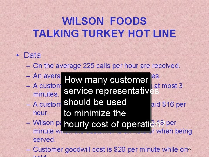
WILSON FOODS TALKING TURKEY HOT LINE • Wilson Foods has an 800 number to answer customers’ questions. • If all the customer representatives are busy when a new customer calls, he/she is asked to stay on the line. • A customer stays on the line if the waiting time is not longer than 3 minutes. 65

WILSON FOODS TALKING TURKEY HOT LINE • Data – On the average 225 calls per hour are received. – An average phone call takes 1. 5 minutes. How many customer – A customer will stay on the line waiting at most 3 minutes. service representatives should used is paid $16 per – A customer service be representative hour. to minimize the – Wilson pays the telephone $0. 18 per hourly cost ofcompany operation? minute when the customer is on hold or when being served. – Customer goodwill cost is $20 per minute while on 66

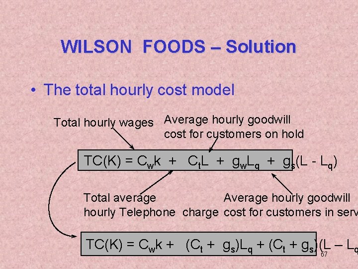
WILSON FOODS – Solution • The total hourly cost model Total hourly wages Average hourly goodwill cost for customers on hold TC(K) = Cwk + Ct. L + gw. Lq + gs(L - Lq) Total average Average hourly goodwill hourly Telephone charge cost for customers in serv TC(K) = Cwk + (Ct + gs)Lq + (Ct + gs)(L – Lq 67

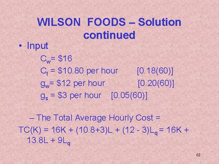
WILSON FOODS – Solution continued • Input Cw= $16 Ct = $10. 80 per hour [0. 18(60)] gw= $12 per hour [0. 20(60)] gs = $3 per hour [0. 05(60)] – The Total Average Hourly Cost = TC(K) = 16 K + (10. 8+3)L + (12 - 3)Lq = 16 K + 13. 8 L + 9 Lq 68

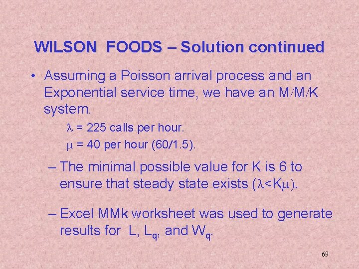
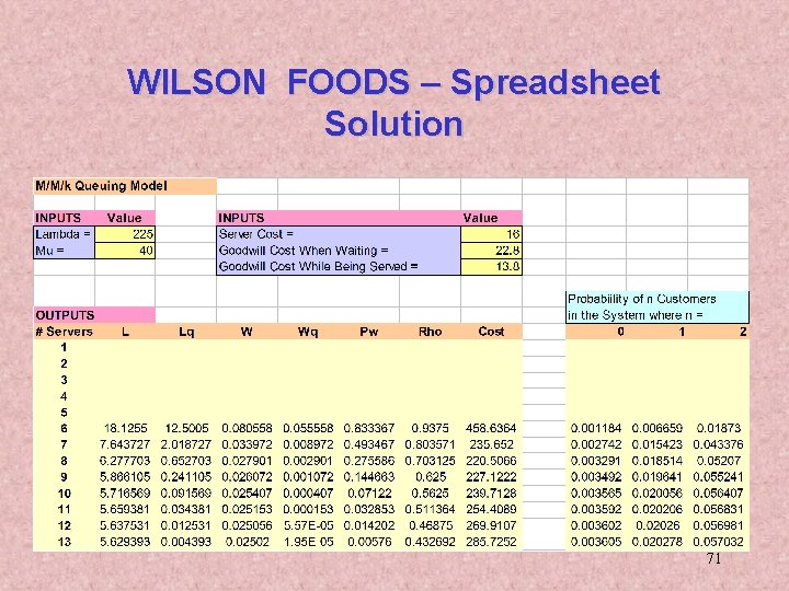
WILSON FOODS – Solution continued • Assuming a Poisson arrival process and an Exponential service time, we have an M/M/K system. l = 225 calls per hour. m = 40 per hour (60/1. 5). – The minimal possible value for K is 6 to ensure that steady state exists (l<Km). – Excel MMk worksheet was used to generate results for L, Lq, and Wq. 69

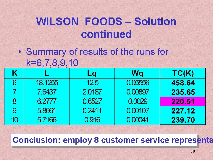
WILSON FOODS – Solution continued • Summary of results of the runs for k=6, 7, 8, 9, 10 Conclusion: employ 8 customer service representa 70

WILSON FOODS – Spreadsheet Solution 71

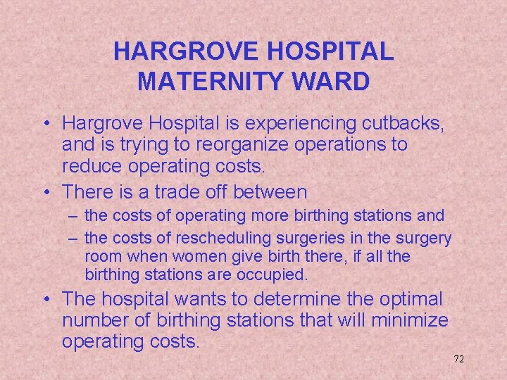
HARGROVE HOSPITAL MATERNITY WARD • Hargrove Hospital is experiencing cutbacks, and is trying to reorganize operations to reduce operating costs. • There is a trade off between – the costs of operating more birthing stations and – the costs of rescheduling surgeries in the surgery room when women give birth there, if all the birthing stations are occupied. • The hospital wants to determine the optimal number of birthing stations that will minimize operating costs. 72

HARGROVE HOSPITAL MATERNITY WARD • Data – Cutting one birthing station saves $25, 000 per year. – Building a birthing station costs $30, 000. – Maternity in the surgery room costs $400 per hour. – Six women on the average need a birthing station a day. The arrival process is Poisson. – Every birthing process occupies a birthing 73

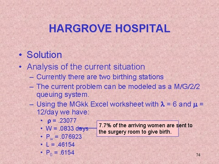
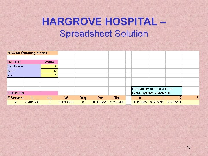
HARGROVE HOSPITAL • Solution • Analysis of the current situation – Currently there are two birthing stations – The current problem can be modeled as a M/G/2/2 queuing system. – Using the MGkk Excel worksheet with l = 6 and m = 12/day we have: • • • r =. 23077 W =. 0833 days Pw =. 076923 L =. 46154 P 0 =. 6154 7. 7% of the arriving women are sent to the surgery room to give birth. 74

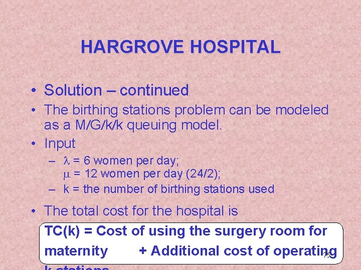
HARGROVE HOSPITAL • Solution – continued • The birthing stations problem can be modeled as a M/G/k/k queuing model. • Input – l = 6 women per day; m = 12 women per day (24/2); – k = the number of birthing stations used • The total cost for the hospital is TC(k) = Cost of using the surgery room for maternity + Additional cost of operating 75

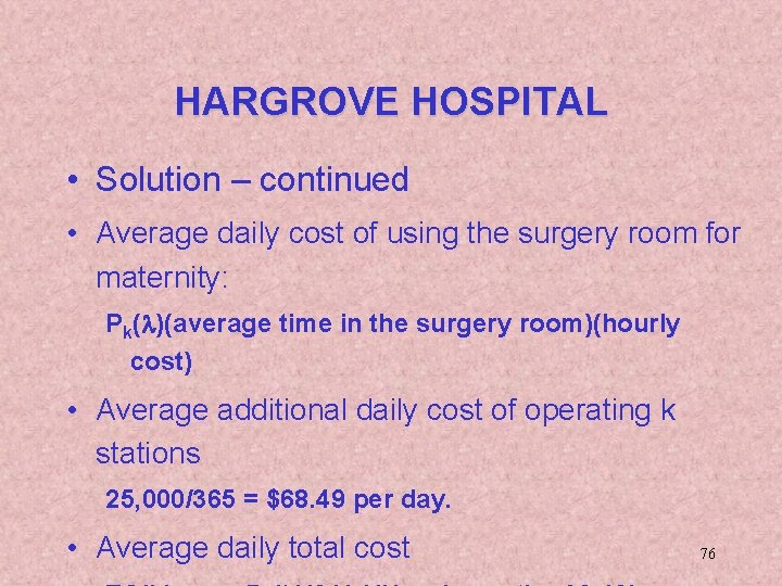
HARGROVE HOSPITAL • Solution – continued • Average daily cost of using the surgery room for maternity: Pk(l)(average time in the surgery room)(hourly cost) • Average additional daily cost of operating k stations 25, 000/365 = $68. 49 per day. • Average daily total cost 76

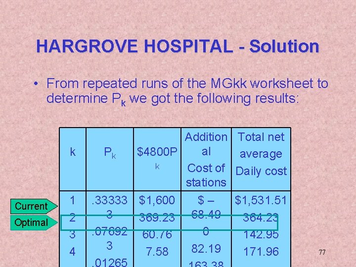
HARGROVE HOSPITAL - Solution • From repeated runs of the MGkk worksheet to determine Pk we got the following results: k Current Optimal 1 2 3 4 Pk Addition Total net al $4800 P average k Cost of Daily cost stations . 33333 $1, 600 3 369. 23. 07692 60. 76 3 7. 58. 01265 $– 68. 49 0 82. 19 $1, 531. 51 364. 23 142. 95 171. 96 77

HARGROVE HOSPITAL – Spreadsheet Solution 78

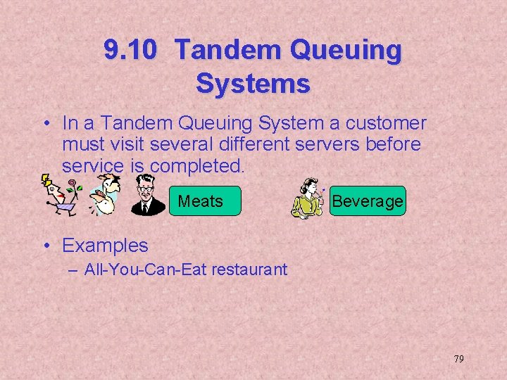
9. 10 Tandem Queuing Systems • In a Tandem Queuing System a customer must visit several different servers before service is completed. Meats Beverage • Examples – All-You-Can-Eat restaurant 79

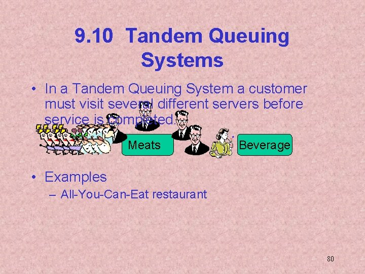
9. 10 Tandem Queuing Systems • In a Tandem Queuing System a customer must visit several different servers before service is completed. Meats Beverage • Examples – All-You-Can-Eat restaurant 80

9. 10 Tandem Queuing Systems • In a Tandem Queuing System a customer must visit several different servers before service is completed. Meats Beverage • Examples – All-You-Can-Eat restaurant – A drive-in restaurant, where first you place your order, then pay and receive it in the next window. – A multiple stage assembly line. 81

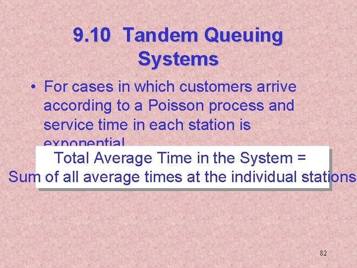
9. 10 Tandem Queuing Systems • For cases in which customers arrive according to a Poisson process and service time in each station is exponential, …. Total Average Time in the System = Sum of all average times at the individual stations 82

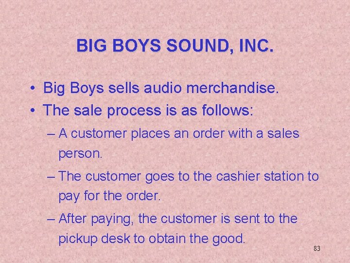
BIG BOYS SOUND, INC. • Big Boys sells audio merchandise. • The sale process is as follows: – A customer places an order with a sales person. – The customer goes to the cashier station to pay for the order. – After paying, the customer is sent to the pickup desk to obtain the good. 83

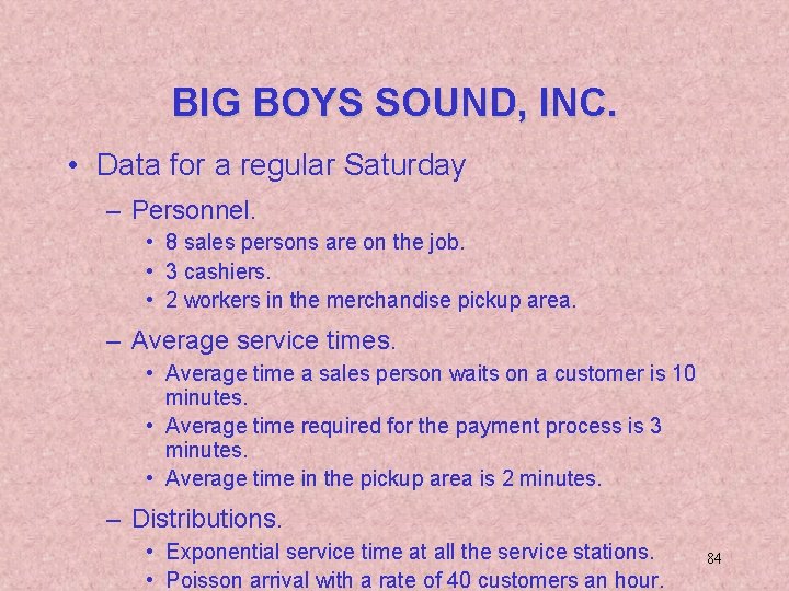
BIG BOYS SOUND, INC. • Data for a regular Saturday – Personnel. • 8 sales persons are on the job. • 3 cashiers. • 2 workers in the merchandise pickup area. – Average service times. • Average time a sales person waits on a customer is 10 minutes. • Average time required for the payment process is 3 minutes. • Average time in the pickup area is 2 minutes. – Distributions. • Exponential service time at all the service stations. • Poisson arrival with a rate of 40 customers an hour. 84

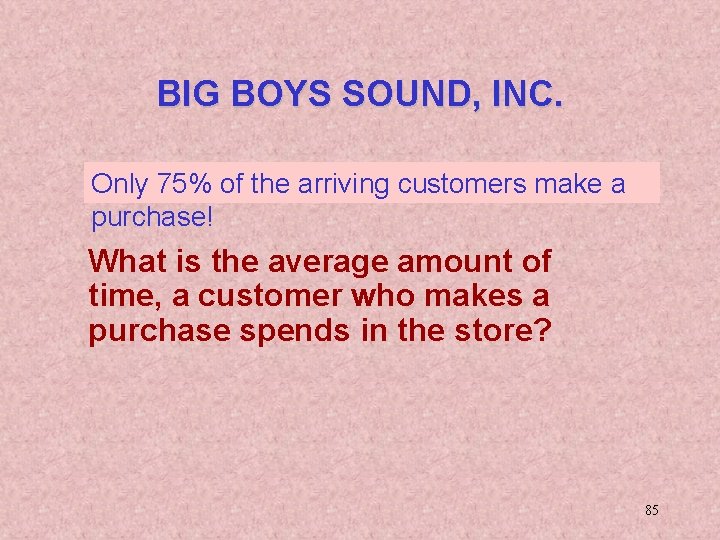
BIG BOYS SOUND, INC. Only 75% of the arriving customers make a purchase! What is the average amount of time, a customer who makes a purchase spends in the store? 85

BIG BOYS SOUND, INC. – Solution • This is a Three Station Tandem Queuing System Pickup desk (. 75)(40)=30 l = 30 Cashiers M/M/3 Sales Clerks M/M/8 M/M/2 l = l W 3 = 2. 67 minutes 40 30 = W 1 = 14 minutes W 2 = 3. 47 minutes Total = 20. 14 minutes 86

Copyright 2002 John Wiley & Sons, Inc. All rights reserved. Reproduction or translation of this work beyond that named in Section 117 of the United States Copyright Act without the express written consent of the copyright owner is unlawful. Requests for further information should be addressed to the Permissions Department, John Wiley & Sons, Inc. Adopters of the textbook are granted permission to make back-up copies for their own use only, to make copies for distribution to students of the course the textbook is used in, and to modify this material to best suit their instructional needs. Under no circumstances can copies be made for resale. The Publisher assumes no responsibility for errors, omissions, or damages, caused by the use of these programs or from the use of the information contained herein. 87