Chapter 9 Profit Maximization Mc GrawHillIrwin Copyright 2008

Chapter 9 Profit Maximization Mc. Graw-Hill/Irwin Copyright © 2008 by The Mc. Graw-Hill Companies, Inc. All Rights Reserved.

Main Topics ¢Profit-maximizing quantities and prices ¢Marginal revenue, marginal cost, and profit maximization ¢Supply decisions by price-taking firms ¢Short-run versus long-run supply ¢Producer surplus 9 -2

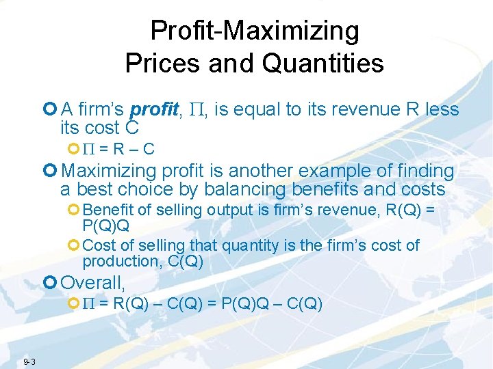
Profit-Maximizing Prices and Quantities ¢ A firm’s profit, P, is equal to its revenue R less its cost C ¢P = R – C ¢ Maximizing profit is another example of finding a best choice by balancing benefits and costs ¢Benefit of selling output is firm’s revenue, R(Q) = P(Q)Q ¢Cost of selling that quantity is the firm’s cost of production, C(Q) ¢ Overall, ¢P = R(Q) – C(Q) = P(Q)Q – C(Q) 9 -3

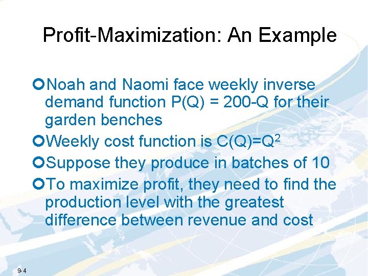
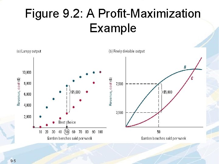
Profit-Maximization: An Example ¢Noah and Naomi face weekly inverse demand function P(Q) = 200 -Q for their garden benches ¢Weekly cost function is C(Q)=Q 2 ¢Suppose they produce in batches of 10 ¢To maximize profit, they need to find the production level with the greatest difference between revenue and cost 9 -4

Figure 9. 2: A Profit-Maximization Example 9 -5

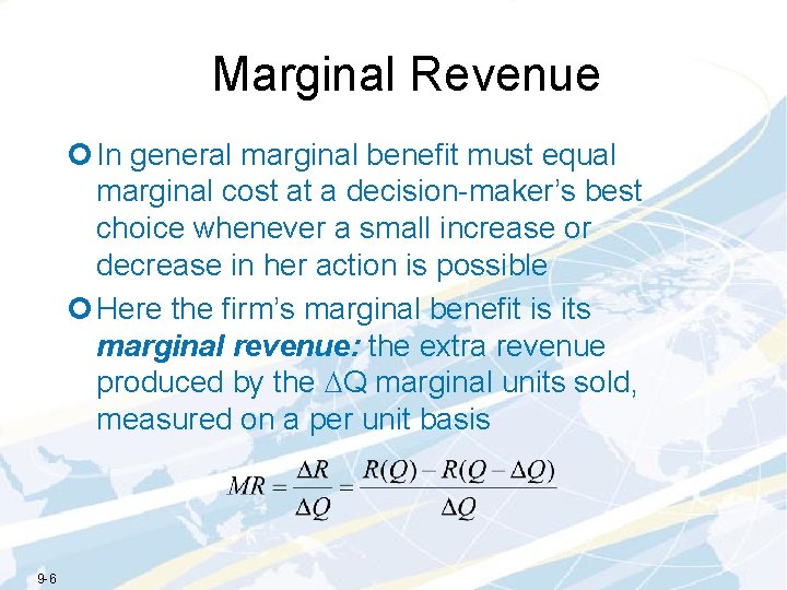
Marginal Revenue ¢ In general marginal benefit must equal marginal cost at a decision-maker’s best choice whenever a small increase or decrease in her action is possible ¢ Here the firm’s marginal benefit is its marginal revenue: the extra revenue produced by the DQ marginal units sold, measured on a per unit basis 9 -6

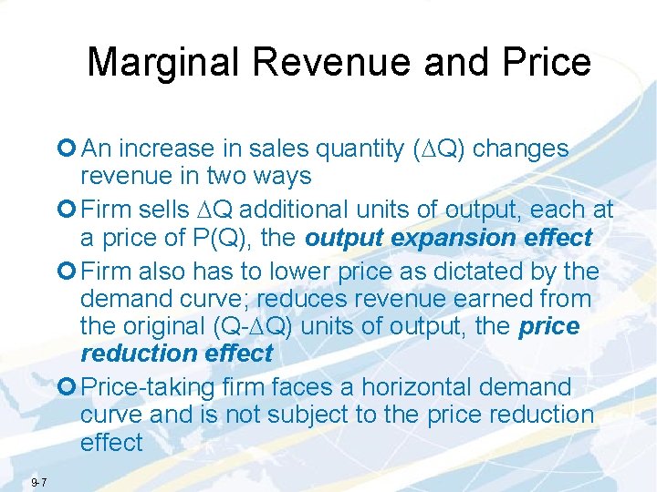
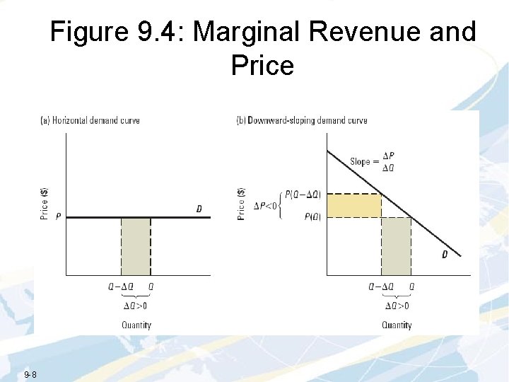
Marginal Revenue and Price ¢ An increase in sales quantity (DQ) changes revenue in two ways ¢ Firm sells DQ additional units of output, each at a price of P(Q), the output expansion effect ¢ Firm also has to lower price as dictated by the demand curve; reduces revenue earned from the original (Q-DQ) units of output, the price reduction effect ¢ Price-taking firm faces a horizontal demand curve and is not subject to the price reduction effect 9 -7

Figure 9. 4: Marginal Revenue and Price 9 -8

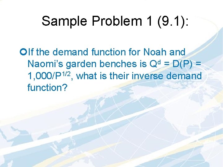
Sample Problem 1 (9. 1): ¢If the demand function for Noah and Naomi’s garden benches is Qd = D(P) = 1, 000/P 1/2, what is their inverse demand function?

Profit-Maximizing Sales Quantity ¢ Two-step procedure for finding the profitmaximizing sales quantity ¢ Step 1: Quantity Rule ¢Identify positive sales quantities at which MR=MC ¢If more than one, find one with highest P ¢ Step 2: Shut-Down Rule ¢Check whether the quantity from Step 1 yields higher profit than shutting down 9 -10

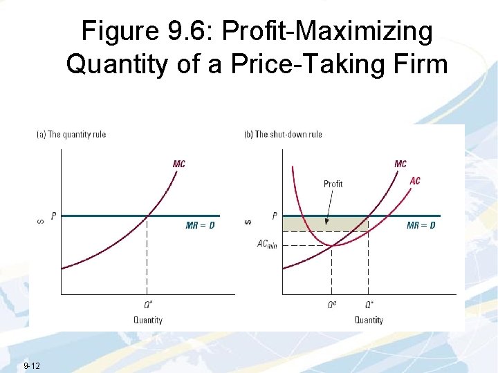
Supply Decisions ¢ Price takers are firms that can sell as much as they want at some price P but nothing at any higher price ¢ Face a perfectly horizontal demand curve ¢ Firms in perfectly competitive markets, e. g. ¢ MR = P for price takers ¢ Use P=MC in the quantity rule to find the profitmaximizing sales quantity for a price-taking firm ¢ Shut-Down Rule: ¢ If P>ACmin, the best positive sales quantity maximizes profit. ¢ If P<ACmin, shutting down maximizes profit. ¢ If P=ACmin, then both shutting down and the best positive sales quantity yield zero profit, which is the best the firm can do. 9 -11

Figure 9. 6: Profit-Maximizing Quantity of a Price-Taking Firm 9 -12

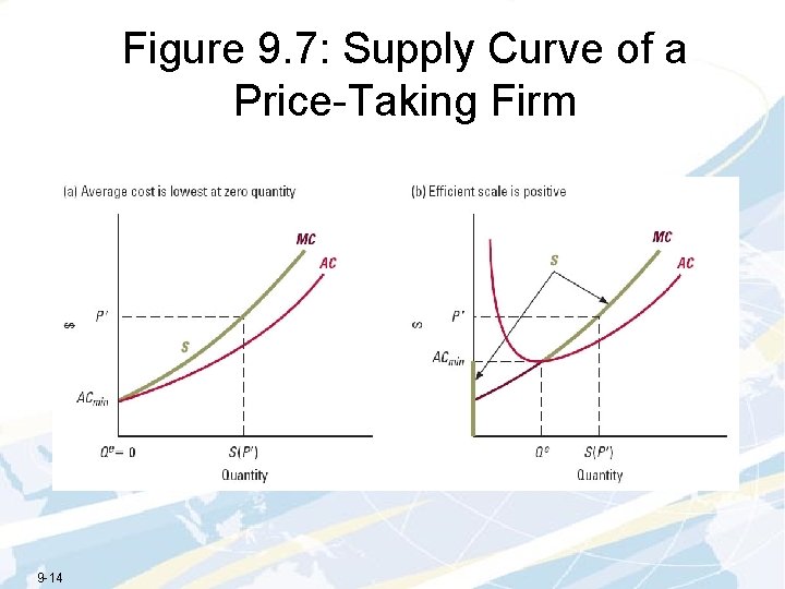
Supply Function of a Price-Taking Firm ¢ A firm’s supply function shows how much it wants to sell at each possible price: Quantity supplied = S(Price) ¢ To find a firm’s supply function, apply the quantity and shut-down rules ¢At each price above ACmin, the firm’s profitmaximizing quantity is positive and satisfies P=MC ¢At each price below ACmin, the firm supplies nothing ¢When price equals ACmin, the firm is indifferent between producing nothing and producing at its efficient scale 9 -13

Figure 9. 7: Supply Curve of a Price-Taking Firm 9 -14

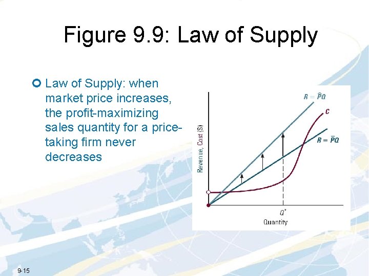
Figure 9. 9: Law of Supply ¢ Law of Supply: when market price increases, the profit-maximizing sales quantity for a pricetaking firm never decreases 9 -15

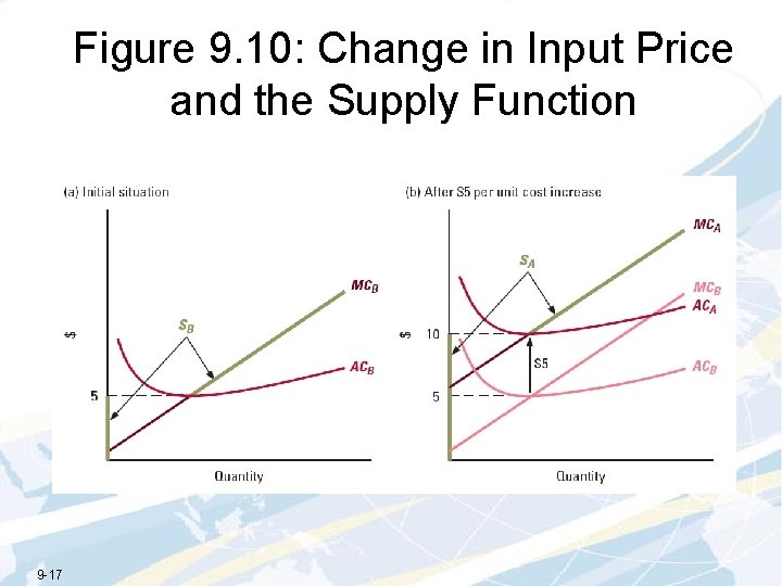
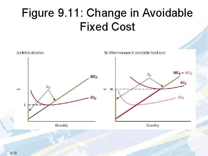
Change in Input Price and the Supply Function ¢ How does a change in an input price affect a firm’s supply function? ¢ Increase in price of an input that raises the per unit cost of production ¢AC, MC curves shift up ¢Supply curve shifts up ¢ Increase in an unavoidable fixed cost ¢AC shifts upward ¢MC unaffected ¢Supply curve does not shift 9 -16

Figure 9. 10: Change in Input Price and the Supply Function 9 -17

Figure 9. 11: Change in Avoidable Fixed Cost 9 -18

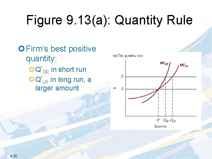
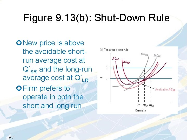
Short-Run versus Long-Run Supply ¢ Firm’s marginal and average costs may differ in the long and short run ¢ This affects firm response over time to a change in the price it faces for its product ¢ Suppose the price rises suddenly and remains at that new high level ¢ Use the quantity and shut-down rules to analyze the long-run and short-run effects of the price increase on the firm’s output 9 -19

Figure 9. 13(a): Quantity Rule ¢ Firm’s best positive quantity: ¢Q*SR in short run ¢Q*LR in long run, a larger amount 9 -20

Figure 9. 13(b): Shut-Down Rule ¢ New price is above the avoidable shortrun average cost at Q*SR and the long-run average cost at Q*LR ¢ Firm prefers to operate in both the short and long run 9 -21

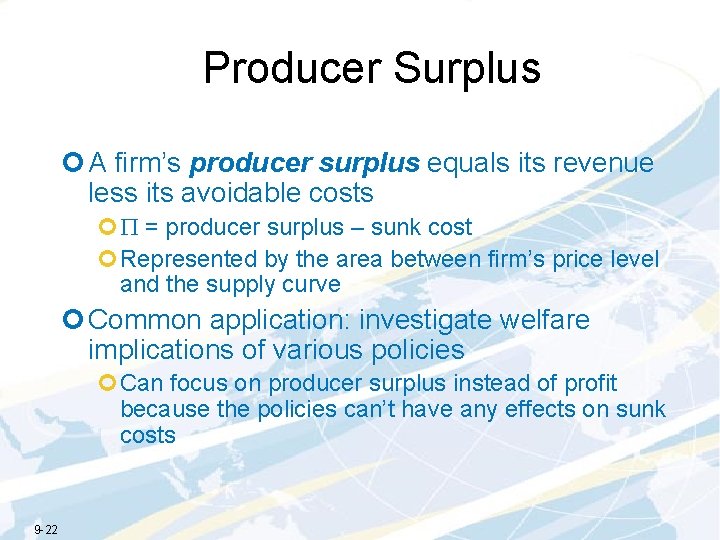
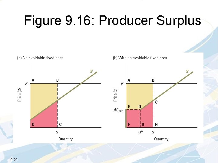
Producer Surplus ¢ A firm’s producer surplus equals its revenue less its avoidable costs ¢P = producer surplus – sunk cost ¢Represented by the area between firm’s price level and the supply curve ¢ Common application: investigate welfare implications of various policies ¢Can focus on producer surplus instead of profit because the policies can’t have any effects on sunk costs 9 -22

Figure 9. 16: Producer Surplus 9 -23

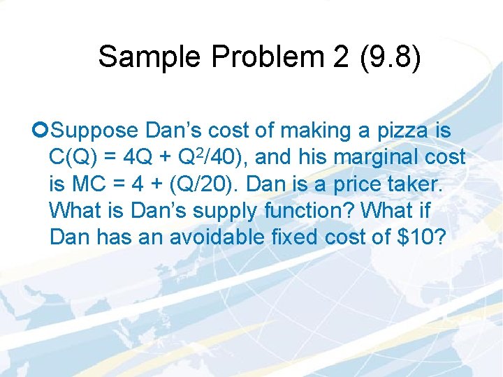
Sample Problem 2 (9. 8) ¢Suppose Dan’s cost of making a pizza is C(Q) = 4 Q + Q 2/40), and his marginal cost is MC = 4 + (Q/20). Dan is a price taker. What is Dan’s supply function? What if Dan has an avoidable fixed cost of $10?