Chapter 9 Linear Programming The Simplex Method To

Chapter 9 Linear Programming: The Simplex Method To accompany Quantitative Analysis for Management, 8 e by Render/Stair/Hanna 9 -1 1

Learning Objectives Students will be able to • Convert LP constraints to equalities with slack, surplus, and artificial variables. • Set up and solve both maximization and minimization LP problems with simplex tableaus. • Interpret the meaning of every number in a simplex tableau. To accompany Quantitative Analysis for Management, 8 e by Render/Stair/Hanna 9 -2 2

Learning Objectives continued Students will be able to • Recognize cases of infeasibility, unboundedness, degeneracy, and multiple optimal solutions in a simplex output. • Understand the relationship between the primal and dual and when to formulate and use the dual. To accompany Quantitative Analysis for Management, 8 e by Render/Stair/Hanna 9 -3 3

Chapter Outline 9. 1 Introduction 9. 2 How to Set Up the Initial Solution 9. 3 Simplex Solution Procedures 9. 4 The Second Simplex Tableau 9. 5 Developing the Third Simplex Tableau To accompany Quantitative Analysis for Management, 8 e by Render/Stair/Hanna 9 -4 4

Chapter Outline continued 9. 6 Review of Procedures for Solving LP Maximization Problems 9. 7 Surplus and Artificial Variables 9. 8 Solving Minimization Problems 9. 9 Review of Procedures for Solving LP Minimization Problems 9. 10 Special Cases To accompany Quantitative Analysis for Management, 8 e by Render/Stair/Hanna 9 -5 5

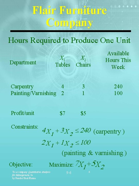
Flair Furniture Company Hours Required to Produce One Unit X 2 Chairs Available Hours This Week Carpentry 4 Painting/Varnishing 2 3 1 240 100 Profit/unit $5 X 1 Tables Department Constraints: $7 4 X 1 + 3 X 2 £ 240 (carpentry ) 2 X 1 + 1 X 2 £ 100 (painting & varnishing ) Objective: Maximize: 7 X 1 +5 X 2 To accompany Quantitative Analysis for Management, 8 e by Render/Stair/Hanna 9 -6 6

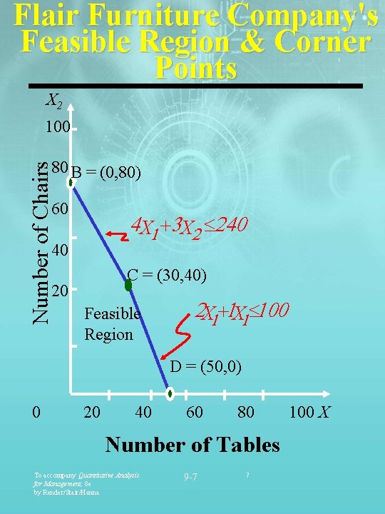
Flair Furniture Company's Feasible Region & Corner Points X 2 100 Number of Chairs 80 B = (0, 80) 60 4 X 1 +3 X 2 £ 240 40 C = (30, 40) 20 Feasible Region 2 X 1+1 X 1£ 100 D = (50, 0) 0 20 40 60 80 Number of Tables To accompany Quantitative Analysis for Management, 8 e by Render/Stair/Hanna 9 -7 7 100 X

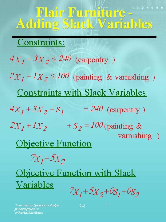
Flair Furniture Adding Slack Variables Constraints: 4 X 1 + 3 X 2 £ 240 (carpentry ) 2 X 1 + 1 X 2 £ 100 (painting & varnishing ) Constraints with Slack Variables 4 X 1 + 3 X 2 + S 1 2 X 1 + 1 X 2 = 240 (carpentry ) + S 2 = 100 (painting & varnishing ) Objective Function 7 X 1 +5 X 2 Objective Function with Slack Variables 7 X 1 +5 X 2 +0 S 1 +0 S 2 To accompany Quantitative Analysis for Management, 8 e by Render/Stair/Hanna 9 -8 8

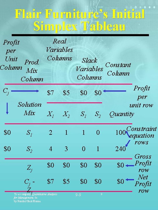
Flair Furniture’s Initial Simplex Tableau Real Profit Variables per Unit Prod. Columns Slack Constant Column Mix Variables Columns Column Cj $7 $5 $0 $0 Solution Mix X 1 X 2 S 1 S 2 $0 S 1 2 1 1 0 $0 S 2 4 3 0 1 Zj $0 $0 Cj $7 $5 Z To accompanyj. Quantitative Analysis $0 $0 for Management, 8 e by Render/Stair/Hanna 9 -9 9 Profit per unit row Quantity Constraint 100 equation rows 240 Gross Profit $0 row Net $0 Profit row

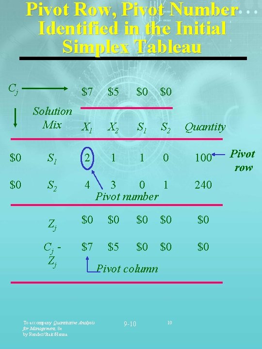
Pivot Row, Pivot Number Identified in the Initial Simplex Tableau Cj $7 $5 $0 $0 Solution Mix X 1 X 2 S 1 S 2 Quantity 1 1 0 100 3 0 1 Pivot number 240 $0 S 1 2 $0 S 2 4 Zj $0 $0 $0 Cj Zj $7 $5 $0 $0 $0 To accompany Quantitative Analysis for Management, 8 e by Render/Stair/Hanna Pivot column 9 -10 10 Pivot row

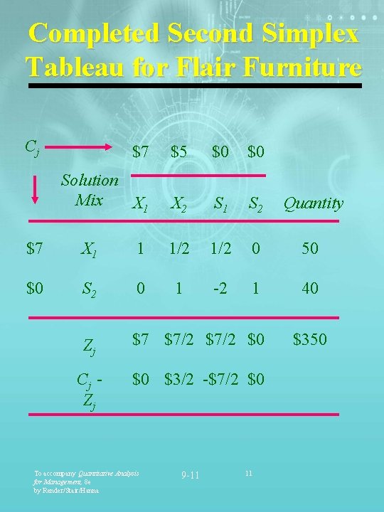
Completed Second Simplex Tableau for Flair Furniture Cj $7 $5 $0 $0 Solution Mix X 1 X 2 S 1 S 2 Quantity $7 X 1 1 1/2 0 50 $0 S 2 0 1 -2 1 40 Zj $7 $7/2 $0 Cj Zj $0 $3/2 -$7/2 $0 To accompany Quantitative Analysis for Management, 8 e by Render/Stair/Hanna 9 -11 11 $350

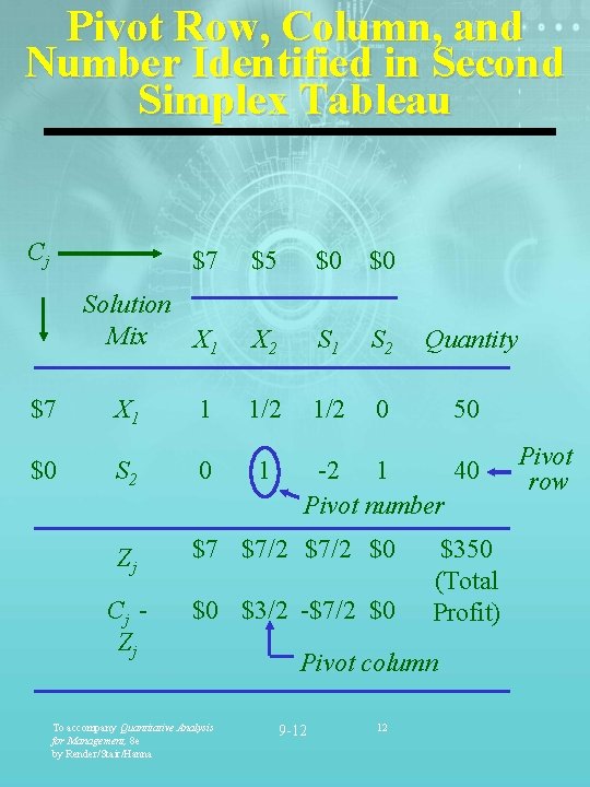
Pivot Row, Column, and Number Identified in Second Simplex Tableau Cj $7 $5 $0 $0 Solution Mix X 1 X 2 S 1 S 2 Quantity 1/2 0 50 $7 X 1 1 1/2 $0 S 2 0 1 Zj $7 $7/2 $0 Cj Zj $0 $3/2 -$7/2 $0 To accompany Quantitative Analysis for Management, 8 e by Render/Stair/Hanna -2 1 40 Pivot number $350 (Total Profit) Pivot column 9 -12 12 Pivot row

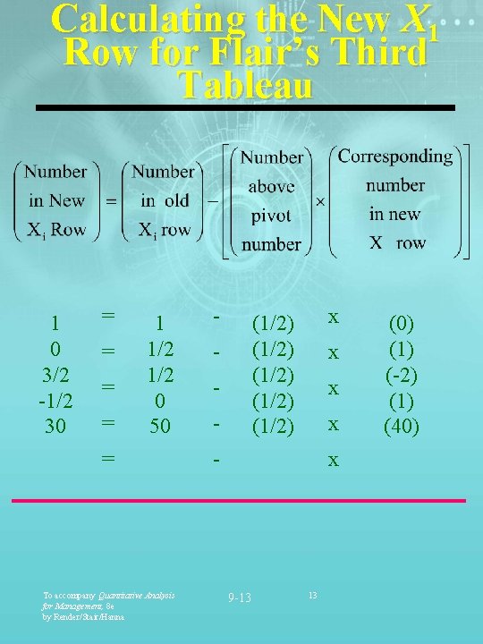
Calculating the New X 1 Row for Flair’s Third Tableau 1 0 3/2 -1/2 30 = = 1 1/2 0 50 = To accompany Quantitative Analysis for Management, 8 e by Render/Stair/Hanna - x (1/2) (1/2) - x x x - x 9 -13 13 (0) (1) (-2) (1) (40)

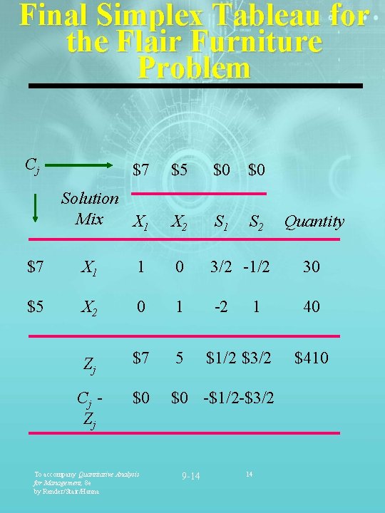
Final Simplex Tableau for the Flair Furniture Problem Cj $7 $5 $0 $0 Solution Mix X 1 X 2 S 1 S 2 Quantity $7 X 1 1 0 3/2 -1/2 30 $5 X 2 0 1 -2 40 Zj $7 5 Cj Zj $0 $0 -$1/2 -$3/2 To accompany Quantitative Analysis for Management, 8 e by Render/Stair/Hanna 9 -14 1 $1/2 $3/2 14 $410

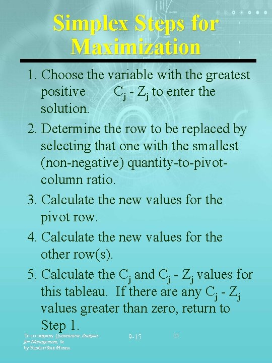
Simplex Steps for Maximization 1. Choose the variable with the greatest positive Cj - Zj to enter the solution. 2. Determine the row to be replaced by selecting that one with the smallest (non-negative) quantity-to-pivotcolumn ratio. 3. Calculate the new values for the pivot row. 4. Calculate the new values for the other row(s). 5. Calculate the Cj and Cj - Zj values for this tableau. If there any Cj - Zj values greater than zero, return to Step 1. To accompany Quantitative Analysis for Management, 8 e by Render/Stair/Hanna 9 -15 15

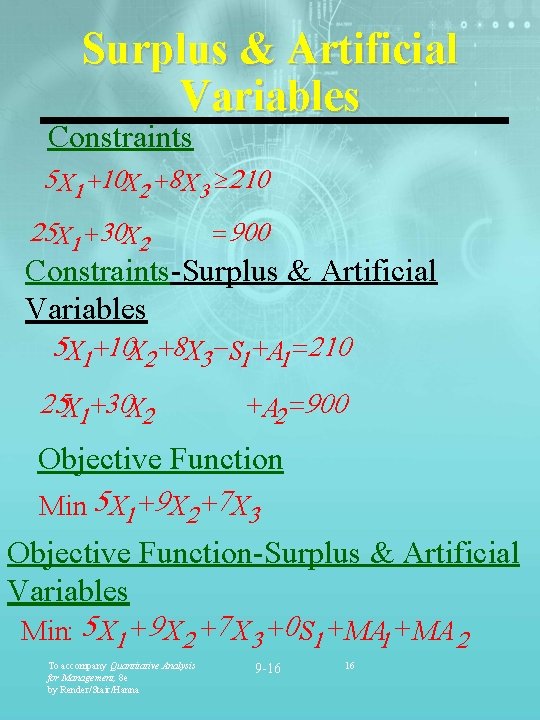
Surplus & Artificial Variables Constraints 5 X 1 +10 X 2 +8 X 3 ³ 210 25 X 1 +30 X 2 = 900 Constraints-Surplus & Artificial Variables 5 X 1 +10 X 2 +8 X 3 -S 1 +A 1 =210 25 X 1 +30 X 2 +A 2 =900 Objective Function Min: 5 X 1 +9 X 2 +7 X 3 Objective Function-Surplus & Artificial Variables Min: 5 X 1 +9 X 2 +7 X 3 +0 S 1 + MA 2 To accompany Quantitative Analysis for Management, 8 e by Render/Stair/Hanna 9 -16 16

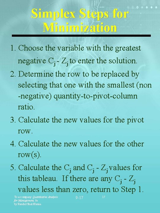
Simplex Steps for Minimization 1. Choose the variable with the greatest negative Cj - Zj to enter the solution. 2. Determine the row to be replaced by selecting that one with the smallest (non -negative) quantity-to-pivot-column ratio. 3. Calculate the new values for the pivot row. 4. Calculate the new values for the other row(s). 5. Calculate the Cj and Cj - Zj values for this tableau. If there any Cj - Zj values less than zero, return to Step 1. To accompany Quantitative Analysis for Management, 8 e by Render/Stair/Hanna 9 -17 17

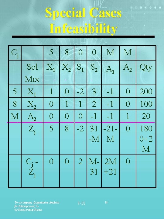
Special Cases Infeasibility Cj 5 8 0 0 M Sol X 1 X 2 S 1 S 2 A 1 Mix 5 X 1 1 0 -2 3 -1 8 X 2 0 1 1 2 -1 M A 2 0 0 0 -1 -1 Zj 5 8 -2 31 -21 -M M Cj Zj 0 To accompany Quantitative Analysis for Management, 8 e by Render/Stair/Hanna 0 2 M- 2 M 31 +21 9 -18 18 M A 2 Qty 0 0 1 0 0 200 100 20 180 0+2 M

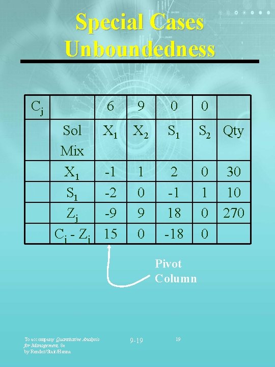
Special Cases Unboundedness Cj 6 9 0 0 Sol X 1 Mix X 1 -1 S 1 -2 Zj -9 Cj - Zj 15 X 2 S 1 S 2 Qty 1 0 9 0 2 -1 18 -18 0 1 0 0 Pivot Column To accompany Quantitative Analysis for Management, 8 e by Render/Stair/Hanna 9 -19 19 30 10 270

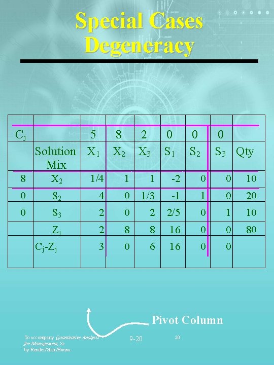
Special Cases Degeneracy Cj 5 Solution X 1 Mix 8 X 2 2 X 3 0 S 1 0 S 2 0 S 3 Qty 8 X 2 1/4 1 1 -2 0 0 10 0 S 2 4 0 1/3 -1 1 0 20 0 S 3 2 0 2 2/5 0 1 10 Zj 2 8 8 16 0 0 80 3 0 6 16 0 0 C j-Z j Pivot Column To accompany Quantitative Analysis for Management, 8 e by Render/Stair/Hanna 9 -20 20

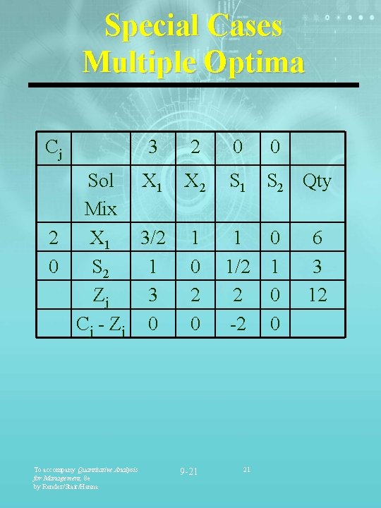
Special Cases Multiple Optima Cj 3 2 0 0 Sol X 1 X 2 S 1 S 2 Qty Mix 2 X 1 3/2 1 1 0 6 0 S 2 1 0 1/2 1 3 Zj 3 2 2 0 12 Cj - Zj 0 0 -2 0 To accompany Quantitative Analysis for Management, 8 e by Render/Stair/Hanna 9 -21 21

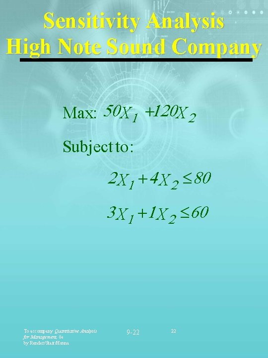
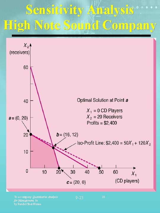
Sensitivity Analysis High Note Sound Company Max: 50 X 1 +120 X 2 Subject to : 2 X 1 + 4 X 2 £ 80 3 X 1 +1 X 2 £ 60 To accompany Quantitative Analysis for Management, 8 e by Render/Stair/Hanna 9 -22 22

Sensitivity Analysis High Note Sound Company To accompany Quantitative Analysis for Management, 8 e by Render/Stair/Hanna 9 -23 23

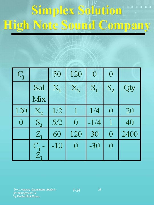
Simplex Solution High Note Sound Company Cj Sol Mix 120 X 2 0 S 2 Zj Cj Zj 50 120 0 0 X 1 X 2 S 1 S 2 Qty 0 1 0 0 20 40 2400 1/2 1 1/4 5/2 0 -1/4 60 120 30 -10 0 -30 To accompany Quantitative Analysis for Management, 8 e by Render/Stair/Hanna 9 -24 24

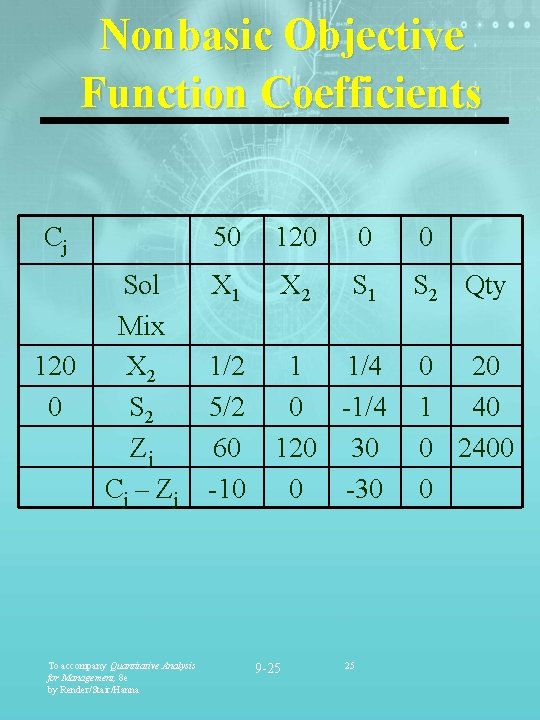
Nonbasic Objective Function Coefficients Cj 120 0 Sol Mix X 2 S 2 Zj Cj – Zj To accompany Quantitative Analysis for Management, 8 e by Render/Stair/Hanna 50 120 0 0 X 1 X 2 S 1 S 2 Qty 1/2 5/2 60 -10 1 1/4 0 -1/4 120 30 0 -30 9 -25 25 0 20 1 40 0 2400 0

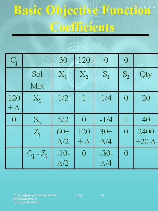
Basic Objective Function Coefficients Cj 120 + 0 Sol Mix X 1 S 2 Zj Cj - Zj 50 120 0 0 X 1 X 2 S 1 S 2 Qty 1/2 1 1/4 0 20 -1/4 30+ /4 -30 /4 1 0 40 2400 +20 5/2 0 60+ 120 /2 + -10 - 0 /2 To accompany Quantitative Analysis for Management, 8 e by Render/Stair/Hanna 9 -26 26 0

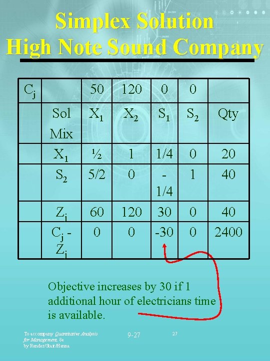
Simplex Solution High Note Sound Company Cj Sol Mix X 1 S 2 Zj Cj Zj 50 120 0 0 X 1 X 2 S 1 S 2 Qty ½ 5/2 1 0 1/4 120 30 0 -30 0 1 20 40 0 0 40 2400 60 0 Objective increases by 30 if 1 additional hour of electricians time is available. To accompany Quantitative Analysis for Management, 8 e by Render/Stair/Hanna 9 -27 27

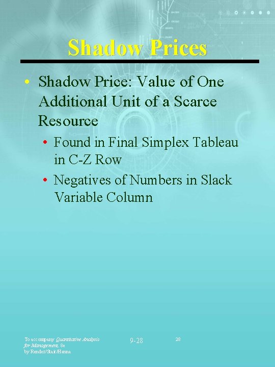
Shadow Prices • Shadow Price: Value of One Additional Unit of a Scarce Resource • Found in Final Simplex Tableau in C-Z Row • Negatives of Numbers in Slack Variable Column To accompany Quantitative Analysis for Management, 8 e by Render/Stair/Hanna 9 -28 28

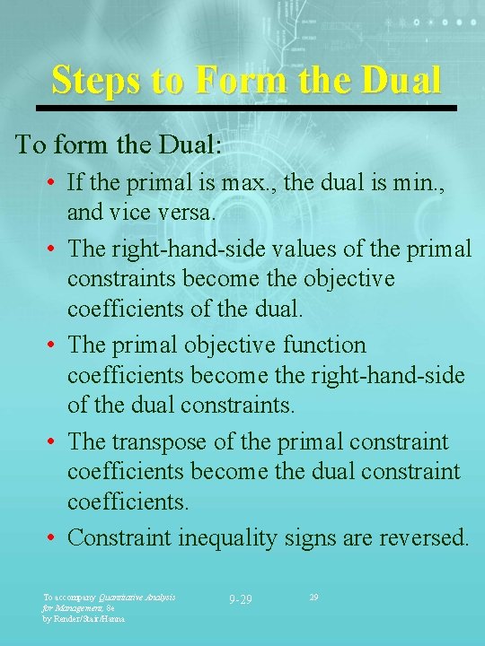
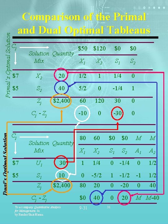
Steps to Form the Dual To form the Dual: • If the primal is max. , the dual is min. , and vice versa. • The right-hand-side values of the primal constraints become the objective coefficients of the dual. • The primal objective function coefficients become the right-hand-side of the dual constraints. • The transpose of the primal constraint coefficients become the dual constraint coefficients. • Constraint inequality signs are reversed. To accompany Quantitative Analysis for Management, 8 e by Render/Stair/Hanna 9 -29 29

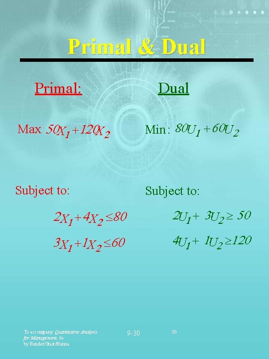
Primal & Dual Primal: Dual Max: 50 X 1 +120 X 2 Min : 80 U 1 + 60 U 2 Subject to: 2 X 1 +4 X 2 £ 80 2 U 1 + 3 U 2 ³ 50 3 X 1 +1 X 2 £ 60 4 U 1 + 1 U 2 ³ 120 To accompany Quantitative Analysis for Management, 8 e by Render/Stair/Hanna 9 -30 30

Primal’s Optimal Solution Comparison of the Primal and Dual Optimal Tableaus Cj $50 $120 Solution Quantity Mix X 1 $0 X 2 S 1 S 2 $7 X 2 20 1/2 1 1/4 0 $5 S 2 40 5/2 0 -1/4 1 Zj $2, 400 60 120 30 0 -10 0 -30 0 80 60 $0 $0 M M X 2 S 1 S 2 A 1 A 2 C j - Zj Dual’s Optimal Solution $0 Cj Solution Quantity Mix X 1 $7 U 1 30 1 1/4 0 -1/4 0 1/2 $5 S 1 10 0 -5/2 1 -1/2 -1 1/2 Zj $2, 400 80 20 0 -20 0 40 $0 40 0 20 M M-40 C j - Zj To accompany Quantitative Analysis for Management, 8 e by Render/Stair/Hanna 9 -31 31