Chapter 9 Introducing Probability 1 From Exploration to

Chapter 9 Introducing Probability 1

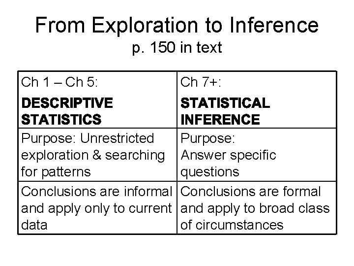
From Exploration to Inference p. 150 in text Ch 1 – Ch 5: Ch 7+: Purpose: Unrestricted exploration & searching for patterns Conclusions are informal and apply only to current data Purpose: Answer specific questions Conclusions are formal and apply to broad class of circumstances

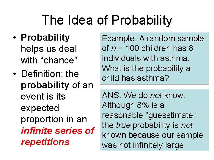
The Idea of Probability • Probability helps us deal with “chance” • Definition: the probability of an event is its expected proportion in an infinite series of repetitions Example: A random sample of n = 100 children has 8 individuals with asthma. What is the probability a child has asthma? ANS: We do not know. Although 8% is a reasonable “guesstimate, ” the true probability is not known because our sample was not infinitely large 3

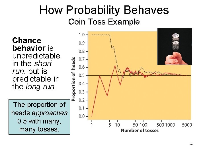
How Probability Behaves Coin Toss Example Chance behavior is unpredictable in the short run, but is predictable in the long run. The proportion of heads approaches 0. 5 with many, many tosses. 4

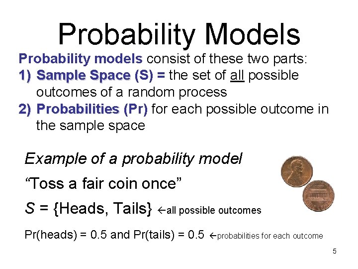
Probability Models Probability models consist of these two parts: 1) Sample Space (S) = the set of all possible outcomes of a random process 2) Probabilities (Pr) for each possible outcome in the sample space Example of a probability model “Toss a fair coin once” S = {Heads, Tails} all possible outcomes Pr(heads) = 0. 5 and Pr(tails) = 0. 5 probabilities for each outcome 5

4 Basic Rules of Probability (Summary) 1. 2. 3. 4. 0 ≤ Pr(A) ≤ 1 Pr(S) = 1 Addition Rule for Disjoint Events Law of Complements Also on bottom of page 1 of Formula Sheet 6

Rule 1 (Range of Possible Probabilities) Let A ≡ event A Pr(A) ≡ probability of event A Rule 1 says “ 0 ≤ Pr(A) ≤ 1” Probabilities are always between 0 & 1 Pr(A) = 0 means A never occurs Pr(A) = 1 means A always occurs Pr(A) =. 25 means A occurs 25% of the time Pr(A) = 1. 25 Impossible! Must be something wrong Pr(A) = some negative number Impossible! Must be something wrong 7

Rule 2 (Sample Space Rule) Let S ≡ the Sample Space Pr(S) = 1 All probabilities in the sample space must sum to 1 exactly. Example: “toss a fair coin” S = {heads or tails} Pr(heads) + Pr(tails) = 0. 5 + 0. 5 = 1. 0 8

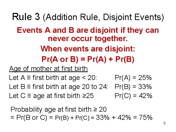
Rule 3 (Addition Rule, Disjoint Events) Events A and B are disjoint if they can never occur together. When events are disjoint: Pr(A or B) = Pr(A) + Pr(B) Age of mother at first birth Let A ≡ first birth at age < 20: Pr(A) = 25% Let B ≡ first birth at age 20 to 24: Pr(B) = 33% Let C ≡ age at first birth ≥ 25 Pr(C) = 42% Probability age at first birth ≥ 20 = Pr(B or C) = Pr(B) + Pr(C) = 33% + 42% = 75% 9

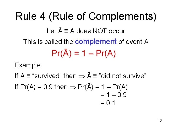
Rule 4 (Rule of Complements) Let Ā ≡ A does NOT occur This is called the complement of event A Pr(Ā) = 1 – Pr(A) Example: If A ≡ “survived” then Ā ≡ “did not survive” If Pr(A) = 0. 9 then Pr(Ā) = 1 – Pr(A) = 1 – 0. 9 = 0. 1 10

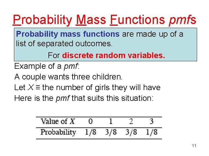
Probability Mass Functions pmfs Probability mass functions are made up of a list of separated outcomes. For discrete random variables. Example of a pmf: A couple wants three children. Let X ≡ the number of girls they will have Here is the pmf that suits this situation: 11

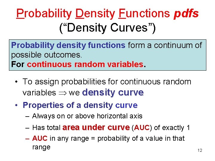
Probability Density Functions pdfs (“Density Curves”) Probability density functions form a continuum of possible outcomes. For continuous random variables. • To assign probabilities for continuous random variables we density curve • Properties of a density curve – Always on or above horizontal axis – Has total area under curve (AUC) AUC of exactly 1 – AUC in any range = probability of a value in that range 12

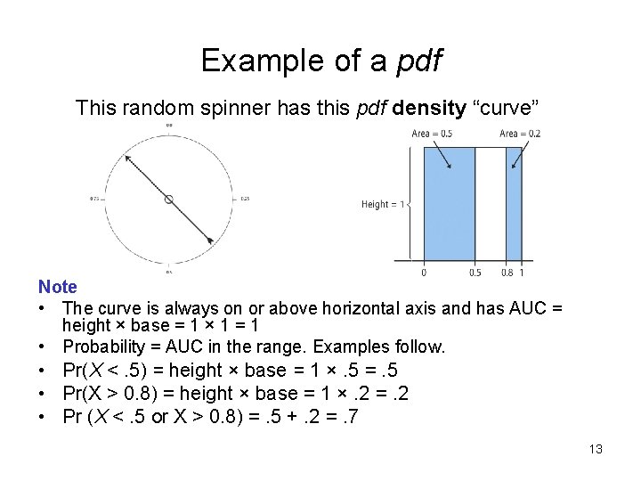
Example of a pdf This random spinner has this pdf density “curve” Note • The curve is always on or above horizontal axis and has AUC = height × base = 1 × 1 = 1 • Probability = AUC in the range. Examples follow. • Pr(X <. 5) = height × base = 1 ×. 5 =. 5 • Pr(X > 0. 8) = height × base = 1 ×. 2 =. 2 • Pr (X <. 5 or X > 0. 8) =. 5 +. 2 =. 7 13

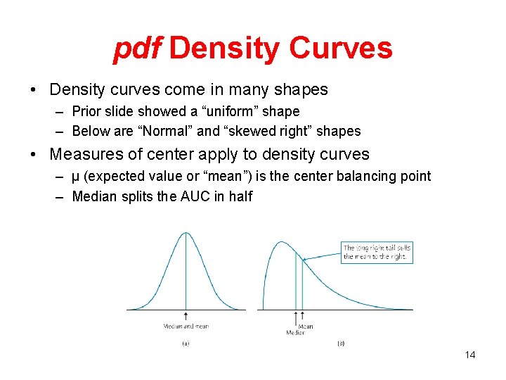
pdf Density Curves • Density curves come in many shapes – Prior slide showed a “uniform” shape – Below are “Normal” and “skewed right” shapes • Measures of center apply to density curves – µ (expected value or “mean”) is the center balancing point – Median splits the AUC in half 14

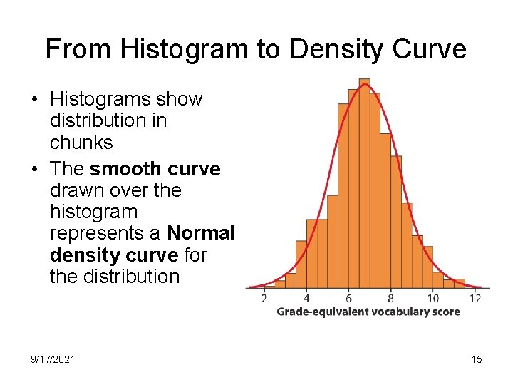
From Histogram to Density Curve • Histograms show distribution in chunks • The smooth curve drawn over the histogram represents a Normal density curve for the distribution 9/17/2021 15

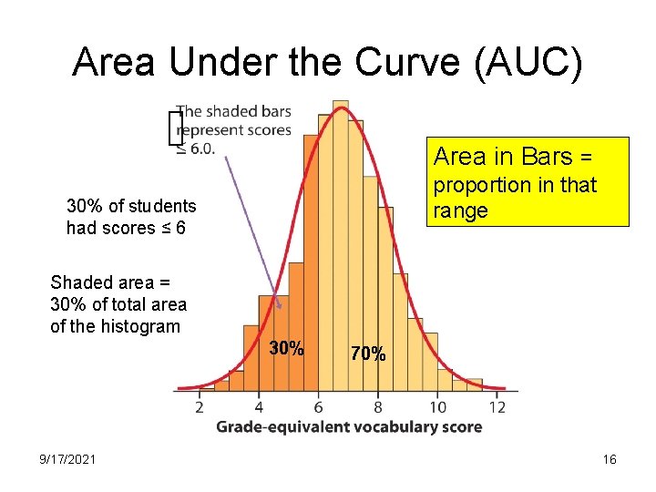
Area Under the Curve (AUC) Area in Bars = proportion in that range 30% of students had scores ≤ 6 Shaded area = 30% of total area of the histogram 30% 9/17/2021 70% 16

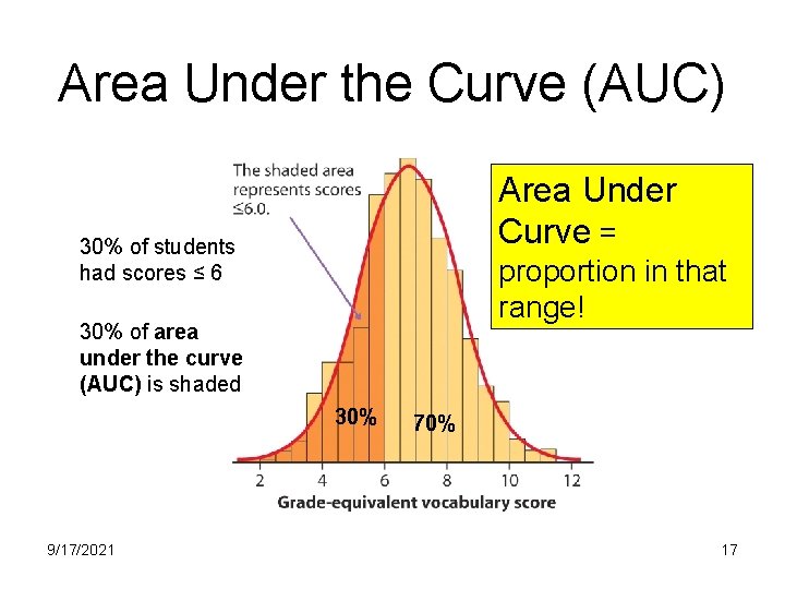
Area Under the Curve (AUC) Area Under Curve = 30% of students had scores ≤ 6 proportion in that range! 30% of area under the curve (AUC) is shaded 30% 9/17/2021 70% 17

Summary of Selected Points • To date we have studied descriptive statistics From here forward we study inferential statistics {2} • Probability is the study chance; chance is unpredictable in the short run but is predictable in the long run {3 - 4}; take the rules of probability to heart{5 - 10} • Discrete random variables are described with probability mass function • Continuous random variables are described with density curves with the area under the curve (AUC) corresponding to probabilities