Chapter 9 Interpreting correlation and regression Fun facts

Chapter 9: Interpreting correlation and regression

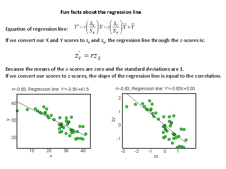
Fun facts about the regression line Equation of regression line: If we convert our X and Y scores to zx and zy, the regression line through the z-scores is: Because the means of the z-scores are zero and the standard deviations are 1. If we convert our scores to z-scores, the slope of the regression line is equal to the correlation. r=-0. 83, Regression line: Y'=-0. 5 X+41. 5 r=-0. 83, Regression line: Y'=-0. 83 X+0. 00 2 40 zy y 1 30 0 20 -1 10 20 x 30 40 -3 -2 -1 0 zx 1

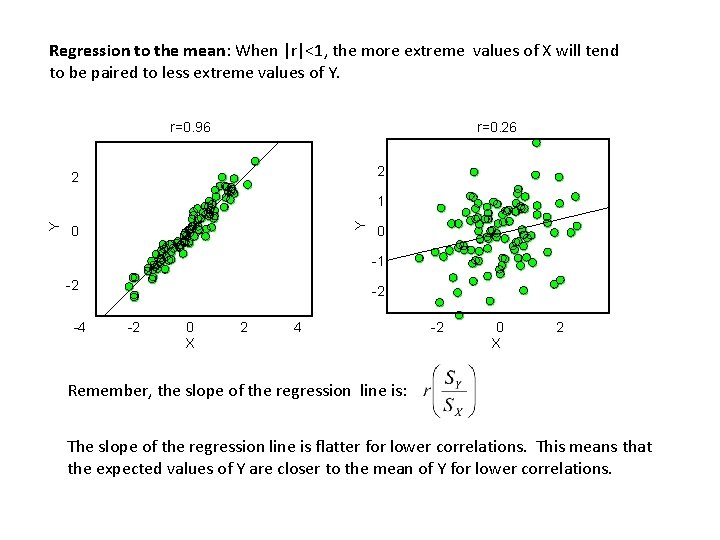
Regression to the mean: When |r|<1, the more extreme values of X will tend to be paired to less extreme values of Y. r=0. 96 r=0. 26 2 2 Y Y 1 0 0 -1 -2 -4 -2 -2 0 X 2 4 -2 0 X 2 Remember, the slope of the regression line is: The slope of the regression line is flatter for lower correlations. This means that the expected values of Y are closer to the mean of Y for lower correlations.

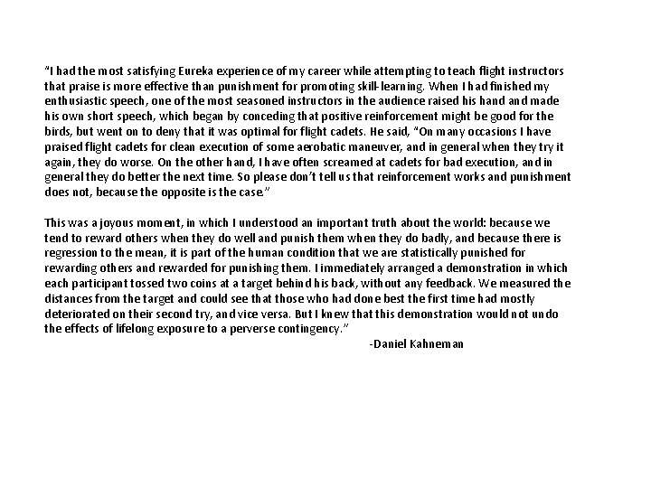
“I had the most satisfying Eureka experience of my career while attempting to teach flight instructors that praise is more effective than punishment for promoting skill-learning. When I had finished my enthusiastic speech, one of the most seasoned instructors in the audience raised his hand made his own short speech, which began by conceding that positive reinforcement might be good for the birds, but went on to deny that it was optimal for flight cadets. He said, “On many occasions I have praised flight cadets for clean execution of some aerobatic maneuver, and in general when they try it again, they do worse. On the other hand, I have often screamed at cadets for bad execution, and in general they do better the next time. So please don’t tell us that reinforcement works and punishment does not, because the opposite is the case. ” This was a joyous moment, in which I understood an important truth about the world: because we tend to reward others when they do well and punish them when they do badly, and because there is regression to the mean, it is part of the human condition that we are statistically punished for rewarding others and rewarded for punishing them. I immediately arranged a demonstration in which each participant tossed two coins at a target behind his back, without any feedback. We measured the distances from the target and could see that those who had done best the first time had mostly deteriorated on their second try, and vice versa. But I knew that this demonstration would not undo the effects of lifelong exposure to a perverse contingency. ” -Daniel Kahneman

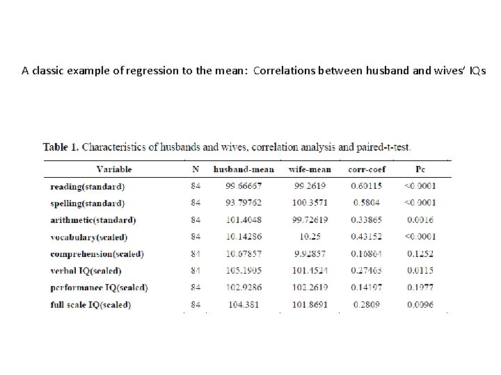
A classic example of regression to the mean: Correlations between husband wives’ IQs

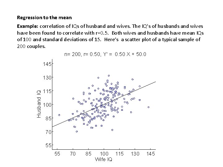
Regression to the mean Example: correlation of IQs of husband wives. The IQ’s of husbands and wives have been found to correlate with r=0. 5. Both wives and husbands have mean IQs of 100 and standard deviations of 15. Here’s a scatter plot of a typical sample of 200 couples. n= 200, r= 0. 50, Y' = 0. 50 X + 50. 0 145 Husband IQ 130 115 100 85 70 55 55 70 85 100 115 Wife IQ 130 145

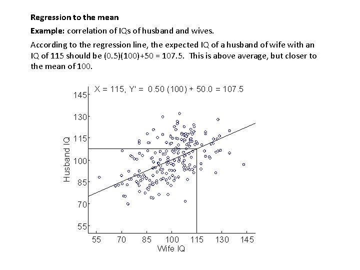
Regression to the mean Example: correlation of IQs of husband wives. According to the regression line, the expected IQ of a husband of wife with an IQ of 115 should be (0. 5)(100)+50 = 107. 5. This is above average, but closer to the mean of 100. 145 X = 115, Y' = 0. 50 (100) + 50. 0 = 107. 5 Husband IQ 130 115 100 85 70 55 55 70 85 100 115 Wife IQ 130 145

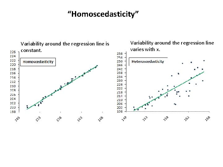
Today’s word: “Homoscedasticity”

“Homoscedasticity” Variability around the regression line is constant. Variability around the regression line varies with x.

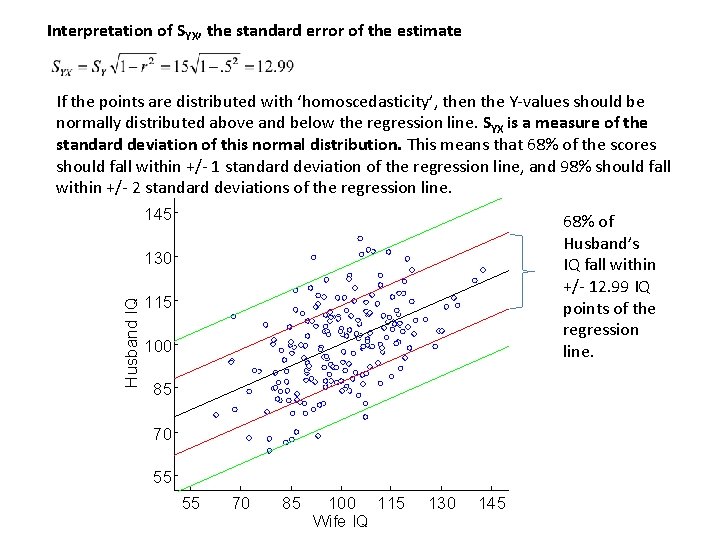
Interpretation of SYX, the standard error of the estimate If the points are distributed with ‘homoscedasticity’, then the Y-values should be normally distributed above and below the regression line. SYX is a measure of the standard deviation of this normal distribution. This means that 68% of the scores should fall within +/- 1 standard deviation of the regression line, and 98% should fall within +/- 2 standard deviations of the regression line. 145 68% of Husband’s IQ fall within +/- 12. 99 IQ points of the regression line. Husband IQ 130 115 100 85 70 55 55 70 85 100 115 Wife IQ 130 145

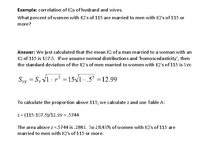
Example: correlation of IQs of husband wives. What percent of women with IQ’s of 115 are married to men with IQ’s of 115 or more? Answer: We just calculated that the mean IQ of a man married to a woman with an IQ of 115 is 107. 5. If we assume normal distributions and ‘homoscedasticity’, then the standard deviation of the IQ’s of men married to women with IQ’s of 115 is S YX: To calculate the proportion above 115, we calculate z and use Table A: z = (115 -107. 5)/12. 99 =. 5744 The area above z =. 5744 is. 2843. So 28. 43% of women with IQ’s of 115 are married to men with IQ’s of 115 or more.

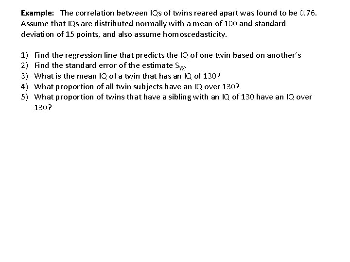
Example: The correlation between IQs of twins reared apart was found to be 0. 76. Assume that IQs are distributed normally with a mean of 100 and standard deviation of 15 points, and also assume homoscedasticity. 1) 2) 3) 4) 5) Find the regression line that predicts the IQ of one twin based on another’s Find the standard error of the estimate SYX. What is the mean IQ of a twin that has an IQ of 130? What proportion of all twin subjects have an IQ over 130? What proportion of twins that have a sibling with an IQ of 130 have an IQ over 130?

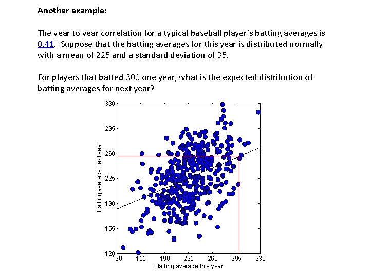
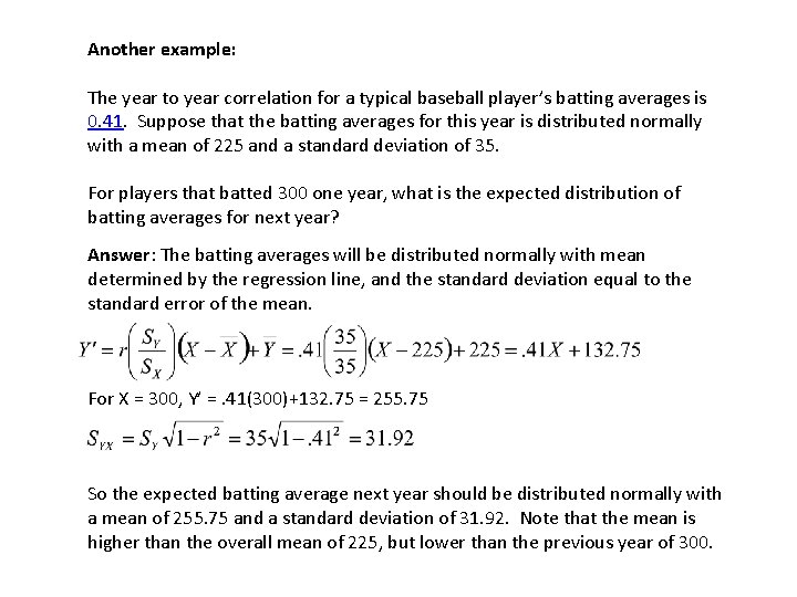
Another example: The year to year correlation for a typical baseball player’s batting averages is 0. 41. Suppose that the batting averages for this year is distributed normally with a mean of 225 and a standard deviation of 35. For players that batted 300 one year, what is the expected distribution of batting averages for next year? 330 Batting average next year 295 260 225 190 155 120 155 190 225 260 Batting average this year 295 330

Another example: The year to year correlation for a typical baseball player’s batting averages is 0. 41. Suppose that the batting averages for this year is distributed normally with a mean of 225 and a standard deviation of 35. For players that batted 300 one year, what is the expected distribution of batting averages for next year? Answer: The batting averages will be distributed normally with mean determined by the regression line, and the standard deviation equal to the standard error of the mean. For X = 300, Y’ =. 41(300)+132. 75 = 255. 75 So the expected batting average next year should be distributed normally with a mean of 255. 75 and a standard deviation of 31. 92. Note that the mean is higher than the overall mean of 225, but lower than the previous year of 300.

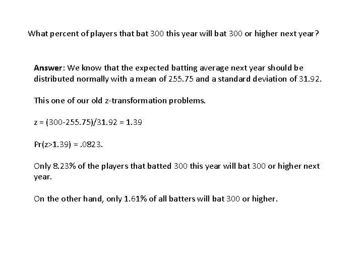
What percent of players that bat 300 this year will bat 300 or higher next year? Answer: We know that the expected batting average next year should be distributed normally with a mean of 255. 75 and a standard deviation of 31. 92. This one of our old z-transformation problems. z = (300 -255. 75)/31. 92 = 1. 39 Pr(z>1. 39) =. 0823. Only 8. 23% of the players that batted 300 this year will bat 300 or higher next year. On the other hand, only 1. 61% of all batters will bat 300 or higher.

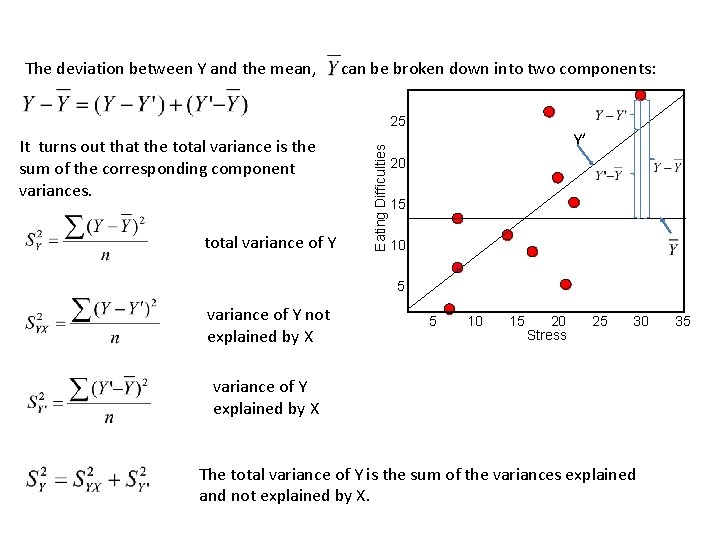
The deviation between Y and the mean, can be broken down into two components: It turns out that the total variance is the sum of the corresponding component variances. total variance of Y Eating Difficulties 25 Y’ 20 15 10 5 variance of Y not explained by X 5 10 15 20 Stress 25 30 variance of Y explained by X The total variance of Y is the sum of the variances explained and not explained by X. 35

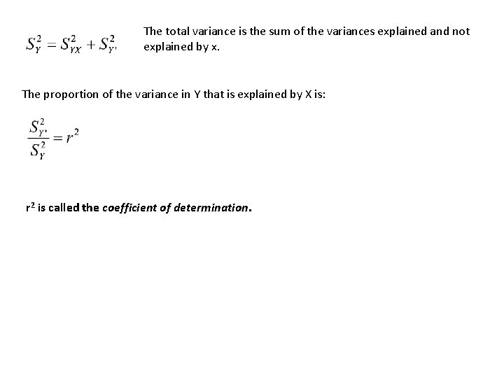
The total variance is the sum of the variances explained and not explained by x. The proportion of the variance in Y that is explained by X is: r 2 is called the coefficient of determination.

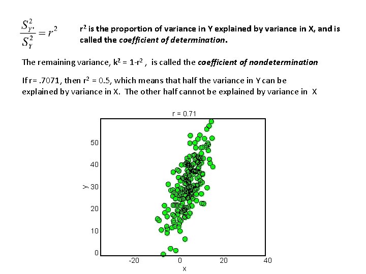
r 2 is the proportion of variance in Y explained by variance in X, and is called the coefficient of determination. The remaining variance, k 2 = 1 -r 2 , is called the coefficient of nondetermination If r=. 7071, then r 2 = 0. 5, which means that half the variance in Y can be explained by variance in X. The other half cannot be explained by variance in X r = 0. 71 50 y 40 30 20 10 0 -20 0 20 x 40

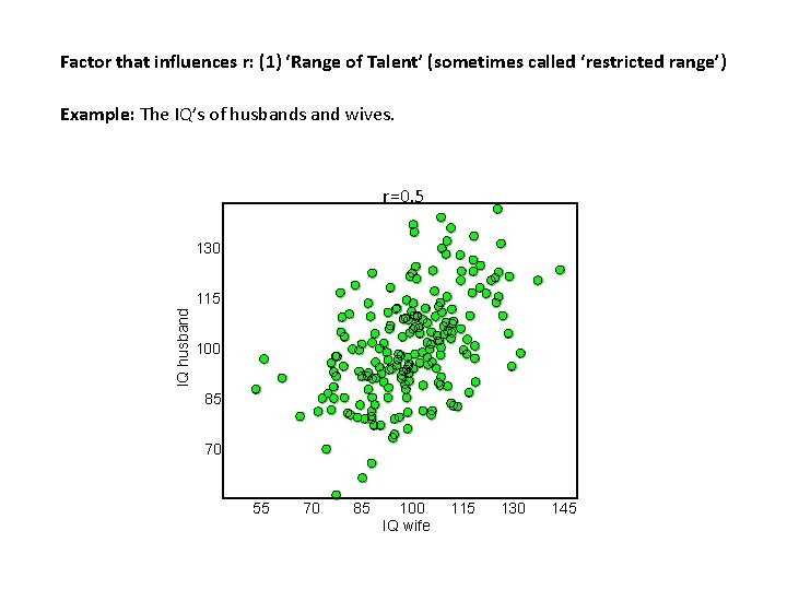
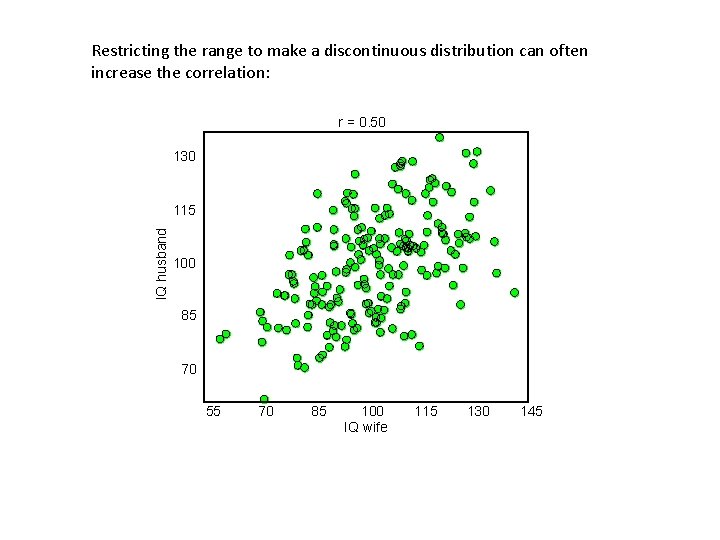
Factor that influences r: (1) ‘Range of Talent’ (sometimes called ‘restricted range’) Example: The IQ’s of husbands and wives. r=0. 5 130 IQ husband 115 100 85 70 55 70 85 100 IQ wife 115 130 145

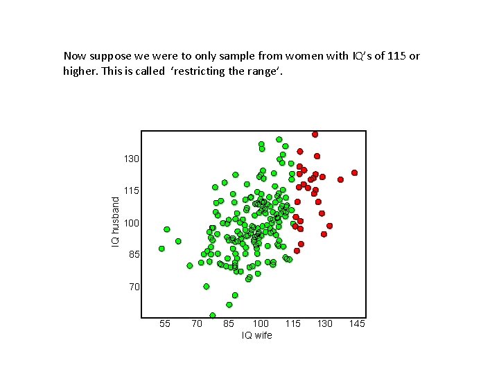
Now suppose we were to only sample from women with IQ’s of 115 or higher. This is called ‘restricting the range’. 130 IQ husband 115 100 85 70 55 70 85 100 IQ wife 115 130 145

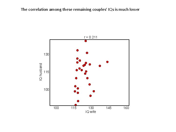
The correlation among these remaining couples’ IQs is much lower r = 0. 211 IQ husband 130 115 100 115 130 IQ wife 145 160

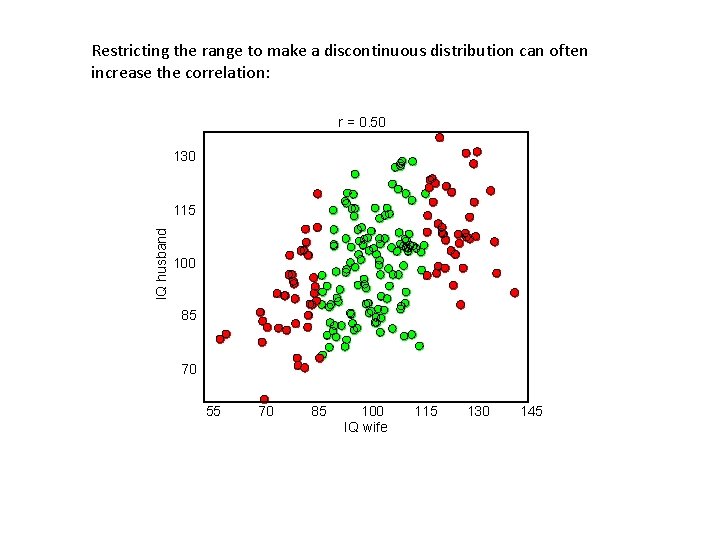
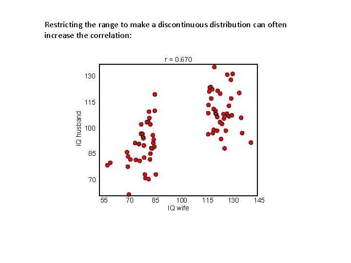
Restricting the range to make a discontinuous distribution can often increase the correlation: r = 0. 50 130 IQ husband 115 100 85 70 55 70 85 100 IQ wife 115 130 145

Restricting the range to make a discontinuous distribution can often increase the correlation: r = 0. 50 130 IQ husband 115 100 85 70 55 70 85 100 IQ wife 115 130 145

Restricting the range to make a discontinuous distribution can often increase the correlation: r = 0. 670 130 IQ husband 115 100 85 70 55 70 85 100 IQ wife 115 130 145

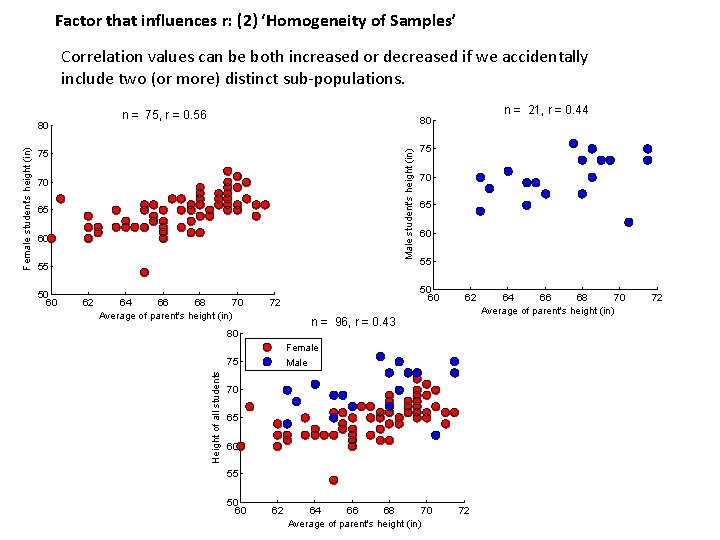
Factor that influences r: (2) ‘Homogeneity of Samples’ Correlation values can be both increased or decreased if we accidentally include two (or more) distinct sub-populations. n = 75, r = 0. 56 Male student's height (in) 75 70 65 60 55 50 60 62 64 66 68 70 Average of parent's height (in) 75 70 65 60 55 50 60 72 62 n = 96, r = 0. 43 80 Female Male 75 Height of all students Female student's height (in) 80 n = 21, r = 0. 44 80 70 65 60 55 50 60 62 64 66 68 70 Average of parent's height (in) 72

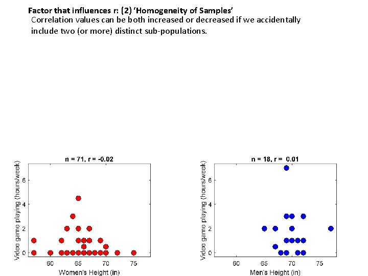
Factor that influences r: (2) ‘Homogeneity of Samples’ Correlation values can be both increased or decreased if we accidentally include two (or more) distinct sub-populations.

Factor that influences r: (2) ‘Homogeneity of Samples’ Correlation values can be both increased or decreased if we accidentally include two (or more) distinct sub-populations.

Factor that influences r: (2) Outliers Just like the mean, extreme values have a large influence on the calculation of correlation.