Chapter 9 FOUNDATIONS OF NEW VENTURE VALUATION Material

Chapter 9 FOUNDATIONS OF NEW VENTURE VALUATION Material from ENTREPRENEURIAL FINANCE: STRATEGY, VALUATION, AND DEAL STRUCTURE, by Janet Kiholm Smith, Richard L. Smith, and Richard T. Bliss, © by Stanford University, all rights reserved. Instructors may make copies of Power. Point Presentation contained herein for classroom distribution only. Any further reproduction, distribution, or use of this material, in any way or by any means, is strictly prohibited without the prior written permission of the publisher.

Learning Objectives • Use the CAPM to value an investment by either the Certainty Equivalent (CEQ) method or the Risk. Adjusted Discount Rate (RADR) method • Use the Relative Value method using accountingbased and non-accounting-based approaches • Use two common venture capital valuation methods: the First Chicago method and the Venture Capital method • Learn how to use each valuation method • Recognize the strengths and weaknesses of each • Learn to correctly match cash flows and discount rates 2

Perspectives on the Valuation of New Ventures • Value of any investment depends on – its ability to generate future cash flows – the riskiness of those cash flows • Challenges specific to new ventures – future cash flows are volatile and difficult to forecast – appropriate discount rates can be tricky to estimate 3

Myths about New Venture Valuation • Myth 3: Investors Demand Very High Rates of Return Source: Timmons, J. A. , and S. Spinelli, Jr. 2007. New Venture Creation: Entrepreneurship for the 21 st Century. 7 th ed. Chicago: Mc. Graw-Hill Irwin 4

Figure 9. 1 5

Perspectives on the Valuation of New Ventures • Historical VC returns (1980 -2004 funds) – average annual IRR = 13. 7% – median annual IRR = 9. 6% – average S&P 500 return = 10. 3% • Sought-for returns are not “expected” returns • Possible explanations for high/low VC returns relative to “expected” – timing, luck, skill, deal flow, unforeseeable events • Two important reasons – valuation mistakes – deal structuring mistakes 6

Myths about New Venture Valuation • Myth 1: Beauty is in the Eye of the Beholder • Myth 2: The Future is Anybody’s Guess • Myth 3: Investors Demand Very High Rates of Return to Compensate Risk • Myth 4: The Investor Determines the Value of the Venture 7

Myths about New Venture Valuation • Myth 3: Investors Demand Very High Rates of Return Source: Timmons, J. A. , and S. Spinelli, Jr. 2007. New Venture Creation: Entrepreneurship for the 21 st Century. 7 th ed. Chicago: Mc. Graw-Hill Irwin 11

Figure 9. 2 12

An Overview of Valuation Methods 1. Discounted cash flow (DCF) - the risk-adjusted discount rate (RADR) approach - the certainty equivalent (CEQ) approach 2. Relative value (RV) 3. The venture capital (VC) method 4. The First Chicago method 14

The Discounted Cash Flow Method • RADR: discount rate reflects riskiness of cash flows and the time value of money – commonly used in corporate finance • CEQ: cash flows are adjusted for risk and then discounted at the risk-free rate – easier to implement than RADR for new ventures • Same result with consistent assumptions 15

The Relative Value (RV) Method • Uses market data on comparable companies or transactions – dimensions of comparability include industry, business model, stage, size, and accounting ratios • Ventures with similar cash flows and risks should have the same value • Widely used for exit strategy valuations – IPO – acquisition 16

The Venture Capital Method • • Popular in the private equity/VC arena Combines elements of DCF and RV methods Based on a successful exit Use a high discount rate to capture – time value – risk – bias of using success-scenario cash flows – dilution from subsequent financing rounds 17

The First Chicago Method • Simplified DCF approach which mitigates some of the problems with the VC method • Uses cash flow estimates for probabilityweighted scenarios • More realistic discount rate • Requires analyst to consider possible outcomes for the venture and their probabilities 18

Discounted Cash Flow Risk-Adjusted Discount Rate 19

DCF Valuation – RADR Approach • Discount rate reflects riskiness of expected cash flows and the time value of money Cjt is the expected future cash flow at time t rt is the risk-adjusted discount rate for a time t cash flow 20

DCF Valuation – RADR Approach • Identifying relevant cash flows • Cash flows an investor expects to receive in exchange for investing – equity dividends – debt interest and principal payments – some securities may have elements of both • preferred stock • convertible bond • Explicit value and continuing value 21

DCF Valuation – RADR Approach • Determining the discount rate r. Ft is the return on a risk-free asset that pays off at time t RPjt is the risk premium RADR discount rate is the opportunity cost the investor could earn on an alternative investment with the same expected return and risk 22

DCF Valuation – RADR Approach • The measure of risk: three equally-likely outcomes Expected holding-period return = [(30% × 1/3) + (15% × 1/3) + (− 10% × 1/3)] = 11. 67% Standard deviation of holding-period return = [(30% − 11. 67%)2 × 1/3 + (15% − 11. 67%)2 × 1/3 + (− 10% − 11. 67%)2 × 1/3]0. 5 = 16. 5% 23

DCF Valuation – RADR Approach • Using the Capital Asset Pricing Model to price risk – Investors’ price for bearing risk – assumptions: • active competition to invest in new ventures • investors view new venture investing as an alternative to other investment opportunities • investors assess project risk based on its contribution to the risk of a diversified portfolio • illiquidity does not affect the investor’s valuation of new venture investment – Allow us to distinguish two types of risk • market, systematic, or nondiversifiable • firm-specific, idiosyncratic, or diversifiable 24

Figure 9. 3 25

Figure 9. 4 26

DCF Valuation – RADR Approach • The CAPM (RADR form) • Beta (of returns) • All measures are based on (equilibrium) holding period returns 27

DCF Valuation – RADR Approach • Relation of holding period returns to future cash flows – RADR approach requires (equilibrium) holding period returns • Requires that you know the PV of risky cash flows or • Or that there be comparable market assets that are priced in the market – May be unlikely for some new ventures – Substituting for rj and βj in Eq. (9. 3) yields 28

Discounted Cash Flow Certainty Equivalent 29

DCF Valuation – Certainty Equivalent Approach The advantage of using the CEQ approach for new ventures • Consider a wager that pays either $1 or $2 with equal probability – How would you calculate - • Expected return • Standard deviation of returns – How would you calculate - • expected payoff • standard deviation of cash flows • To use the RADR approach we need the standard deviation of (equilibrium) holding period returns 30

DCF Valuation – Certainty Equivalent Approach The advantage of using the CEQ approach for new ventures • Consider a wager that pays either $1 or $2 with equal probability – expected payoff is [($1 × 0. 5) + ($2 × 0. 5)] = $1. 50 – standard deviation of cash flows is [($1 − $1. 50)2 × 0. 5 + ($2 − $1. 50)2 × 0. 5]0. 5 = $0. 50 • To use the CEQ approach we do not need the standard deviation of holding period returns 31

DCF Valuation – Certainty Equivalent Approach The challenge of using the RADR approach • What if it costs $1. 25 to acquire the wager? – $1 payoff is a -20% return and a $2 payoff is a 60% return – expected holding-period return is [(-20% × 0. 5) + (60% × 0. 5)] = 20%. – standard deviation of holding period return is [(60% − 20%)2 × 0. 5 + (− 20%)2 × 0. 5]0. 5 = 40% 32

DCF Valuation – Certainty Equivalent Approach The challenge of using the RADR approach • But, what if the cost of the wager is $1. 50 – $1 payoff is a -33% return and a $2 payoff is a 33% return – The expected (mean) holding-period return is [(-33% × 0. 5) + (33% × 0. 5)] = 0% – The realized standard deviation of holding period return is [(-33% − 0%)2 × 0. 5 + (33% − 0%)2 × 0. 5]0. 5 = 33% The expected (mean) return and risk depend on the cost of the wager 33

DCF Valuation – Certainty Equivalent Approach The challenge of using the RADR approach • In corporate settings, problems are finessed by – finding a comparable market asset that is publicly traded – estimate the beta of the market asset – discount project cash flows using that beta in the CAPM • Problem: many new ventures do not have analogous market assets 34

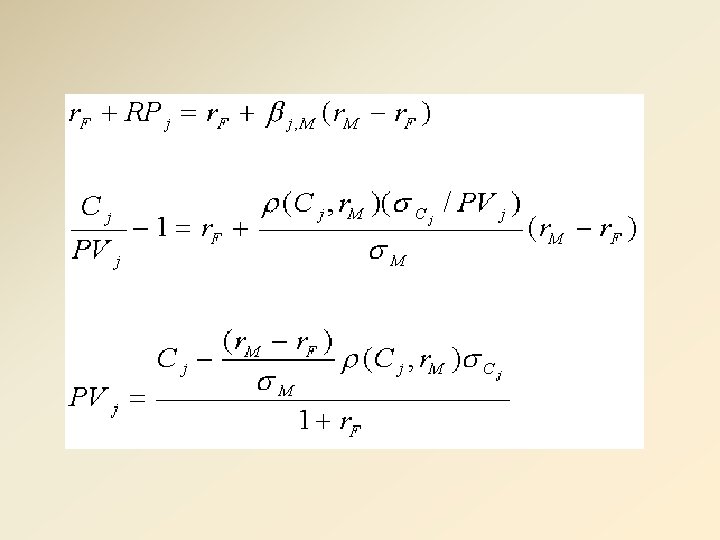
DCF Valuation – Certainty Equivalent Approach • Certainty equivalent of a risky cash flow is the certain cash flow that is equally valuable to the investor • For risk averse investors, the certainty equivalent is less than the expected risky cash flow where CE(Cjt) is the certainty equivalent of the period t expected risky cash flow, Cjt, and RDjt represents the dollarvalued discount to Cjt 35

DCF Valuation – Certainty Equivalent Approach where r. Ft is the risk-free rate for period t cash flows We can solve Eqn. (9. 5) for PVj which is the CEQ form of the CAPM 37

DCF Valuation – Certainty Equivalent Approach • Let’s revisit the wager that pays either $1 or $2 with equal probability with the following assumptions: – risk-free rate is 4. 0% – market risk premium is 6. 0% – standard deviation of holding-period returns of the market portfolio is 20% – correlation between the payoff of the bet and the market portfolio 0. 6 Using Eqn. (9. 8) 38

DCF Valuation – Certainty Equivalent Approach • CEQ cash flow of the expected (risky) $1. 50 is $1. 41 • Discounting at the risk-free rate give a PV of $1. 356 • If it costs $1. 25 to acquire the wager, the NPV is NPV = ($1. 356 - $1. 25) = $0. 106 • If it costs $1. 50 to acquire the wager, the NPV is NPV = ($1. 356 - $1. 50) = -$0. 144 • With a PV of $1. 356, the correct discount rate is (Cj/PVj) − 1 = $1. 50/$1. 356 – 1 = 0. 1062 = 10. 62% 39

Venture Capital Method 40

Valuation by the Venture Capital Method Step 1: Select a terminal year for the valuation by determining a point where harvesting would be feasible Step 2: Develop a success-scenario forecast of cash flow, earnings, or another appropriate measure Step 3: Use the appropriate P-E or other measure and cash flow projection to compute continuing value Step 4: Convert the continuing value estimate to present value by discounting at a hurdle rate 41

Relative Value Method 42

The Relative Value (RV) Method • You are considering the purchase of a threebedroom, 2, 500 -square-foot house with an asking price of $450, 000 and assessed at $439, 000 • You collect the following data on comparable sales: 43

The Relative Value (RV) Method 44

The Relative Value (RV) Method Relative valuation and new ventures • Accounting-based approaches – equity value • Price/earnings, price/BV of equity, price/cash flow – enterprise value (EV) • EV/EBITDA, EV/revenue, EV/BV (equity + debt) • Incorporating growth expectations – P E(1+g)/(r-g) – PEG ratio (P/E to growth) – EV/(EBITDA/growth) • Non-accounting-based approaches 45

First Chicago Method 46

Valuation by the First Chicago Method Step 1: Select a terminal year for the valuation based on likely harvest date in the event of success Step 2: Estimate the cash flows of success, moderate and failure scenarios Step 3: Compute the continuing value by applying a multiplier to each financial projection Step 4: Compute the expected cash flow by weighting each scenario Step 5: Compute PV by discounting the expected CFs 47

Valuation – First Chicago Method • The measure of risk: three equally-likely outcomes – current price (P 0) is $20. Expected cash flow = [($26 × 1/3) + ($23 × 1/3) + ($18 × 1/3)] = $22. 33 Projected return = $22. 33/$20 = 10. 17% Is this a positive NPV? Same as DCF – RADR Approach with discrete scenarios 48

Reconciliation with the Pricing of Options • In the Black-Scholes Option Pricing Model (OPM), value increases with greater risk • Applying the OPM to new venture valuation – OPM assumes complete market and continuous trading • reasonable for public companies, but not new ventures • substituting a “tracking portfolio” for the new venture probably underestimates the risk due to diversification – a new venture typically has numerous complex and interrelated real options, which can make using the OPM impractical 49

Required Rates of Return for Investing in New Ventures • CAPM says that only market risk matters • What does this imply for new ventures? – Much of the risk in new ventures is diversifiable (firm-specific) • a single biotech firm is like a lottery ticket • portfolio of 100 biotech firms has a beta of 0. 75 • betas for new ventures are in the 1. 0 -2. 0 range – With a 4% risk-free rate and 8% market risk premium the CAPM suggests returns between 12% and 20% 50

Required Rates of Return for Investing in New Ventures • Can we reconcile CAPM returns with VC returns? • If gross VC returns are 25 -30%, the GP will take a 2. 5% management fee and 20% of the gains (for effort) • This implies a negligible return for illiquidity, which is supported by recent empirical evidence • CAPM reasonably estimates actual VC returns 51

Matching Cash Flows and Discount Rates • Valuation cash flows are tied to specific financial claims • What is being valued? – debt – equity – enterprise • Discount rates should match the cash flows and also account for capital structure and taxes 52

Table 9. 1 53

Table 9. 2 54

Foundations of New Venture Valuation - Summary • Value is a function of cash flows and risk • Valuation is an important tool for both entrepreneurs and investors and is a critical part of any negotiation • Valuation methods – – DCF (RADR and CEQ) relative value the venture capital method the First Chicago method • Reconciliation with option pricing • Returns for investing in new ventures • Matching cash flows and discount rates 55