Chapter 9 Correlation and Regression LarsonFarber 4 th

Chapter 9 Correlation and Regression Larson/Farber 4 th ed. 1

Correlation • A relationship between two variables. • The data can be represented by ordered pairs (x, y) § x is the independent (or explanatory) variable § y is the dependent (or response) variable Larson/Farber 4 th ed. 2

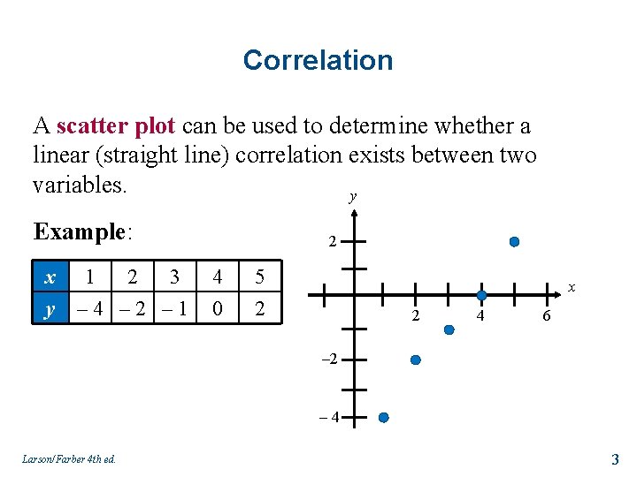
Correlation A scatter plot can be used to determine whether a linear (straight line) correlation exists between two variables. y Example: x y 1 2 3 – 4 – 2 – 1 2 4 0 5 2 x 2 4 6 – 2 – 4 Larson/Farber 4 th ed. 3

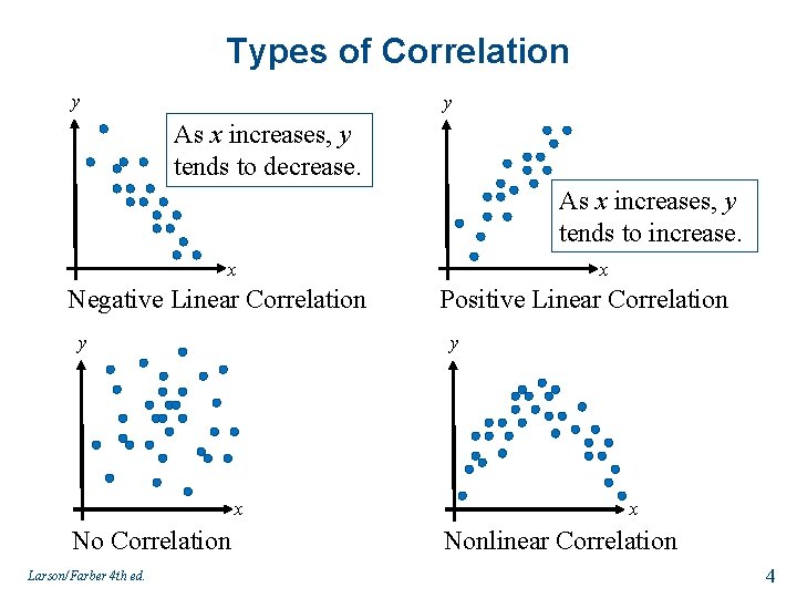
Types of Correlation y y As x increases, y tends to decrease. As x increases, y tends to increase. x x Negative Linear Correlation y y x No Correlation Larson/Farber 4 th ed. Positive Linear Correlation x Nonlinear Correlation 4

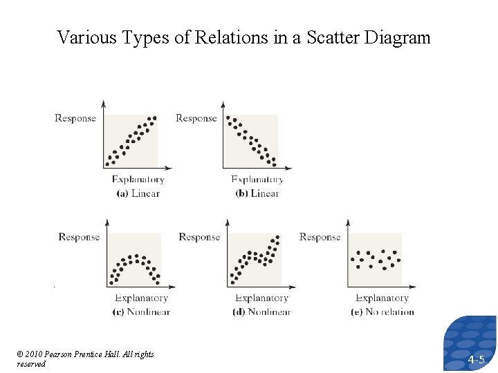
Various Types of Relations in a Scatter Diagram © 2010 Pearson Prentice Hall. All rights reserved 4 -5

© 2010 Pearson Prentice Hall. All rights reserved 4 -6

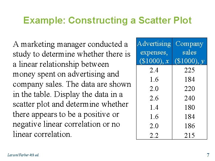
Example: Constructing a Scatter Plot A marketing manager conducted a Advertising Company sales study to determine whethere is expenses, ($1000), x ($1000), y a linear relationship between 2. 4 225 money spent on advertising and 1. 6 184 company sales. The data are shown 2. 0 220 in the table. Display the data in a 2. 6 240 scatter plot and determine whether 1. 4 180 there appears to be a positive or 1. 6 184 negative linear correlation or no 2. 0 186 linear correlation. 2. 2 215 Larson/Farber 4 th ed. 7

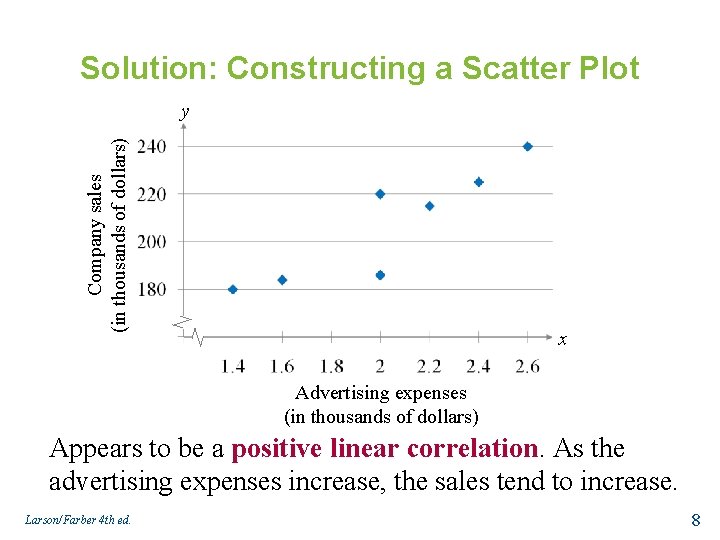
Solution: Constructing a Scatter Plot Company sales (in thousands of dollars) y x Advertising expenses (in thousands of dollars) Appears to be a positive linear correlation. As the advertising expenses increase, the sales tend to increase. Larson/Farber 4 th ed. 8

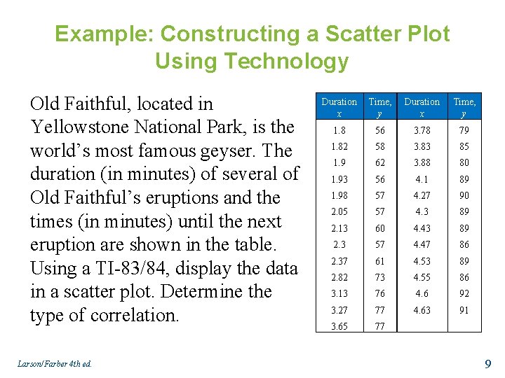
Example: Constructing a Scatter Plot Using Technology Old Faithful, located in Yellowstone National Park, is the world’s most famous geyser. The duration (in minutes) of several of Old Faithful’s eruptions and the times (in minutes) until the next eruption are shown in the table. Using a TI-83/84, display the data in a scatter plot. Determine the type of correlation. Larson/Farber 4 th ed. Duration x Time, y 1. 8 56 3. 78 79 1. 82 58 3. 83 85 1. 9 62 3. 88 80 1. 93 56 4. 1 89 1. 98 57 4. 27 90 2. 05 57 4. 3 89 2. 13 60 4. 43 89 2. 3 57 4. 47 86 2. 37 61 4. 53 89 2. 82 73 4. 55 86 3. 13 76 4. 6 92 3. 27 77 4. 63 91 3. 65 77 9

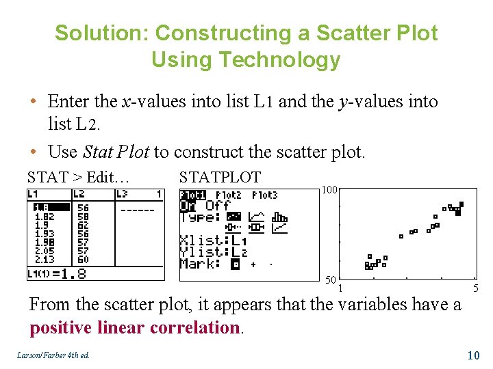
Solution: Constructing a Scatter Plot Using Technology • Enter the x-values into list L 1 and the y-values into list L 2. • Use Stat Plot to construct the scatter plot. STAT > Edit… STATPLOT 100 50 1 From the scatter plot, it appears that the variables have a positive linear correlation. Larson/Farber 4 th ed. 5 10

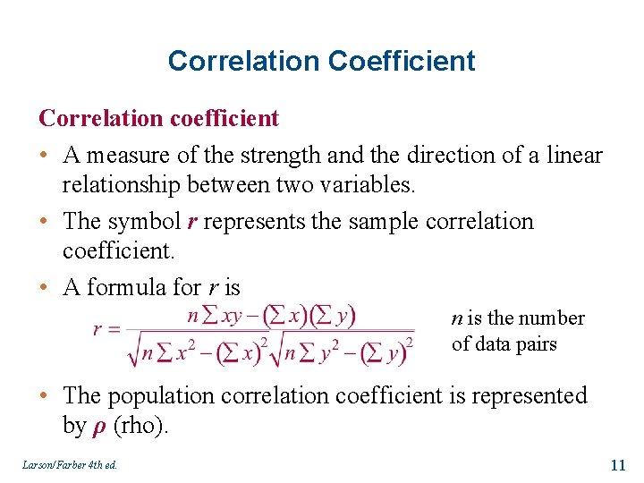
Correlation Coefficient Correlation coefficient • A measure of the strength and the direction of a linear relationship between two variables. • The symbol r represents the sample correlation coefficient. • A formula for r is n is the number of data pairs • The population correlation coefficient is represented by ρ (rho). Larson/Farber 4 th ed. 11

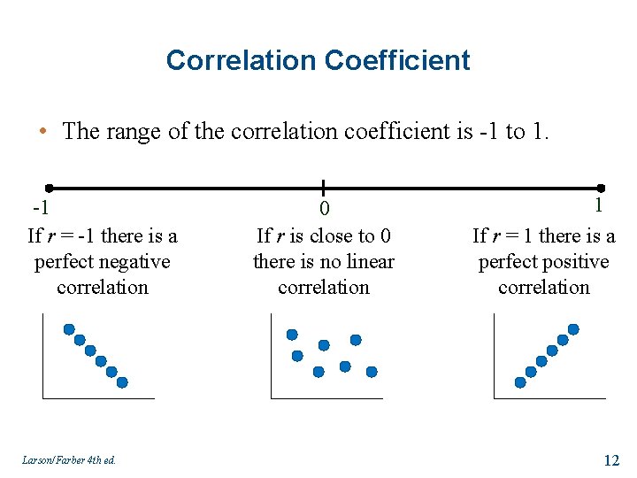
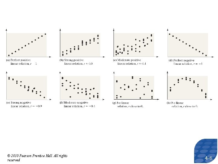
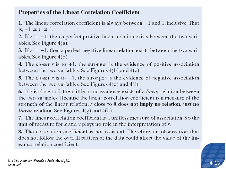
Correlation Coefficient • The range of the correlation coefficient is -1 to 1. -1 If r = -1 there is a perfect negative correlation Larson/Farber 4 th ed. 0 If r is close to 0 there is no linear correlation 1 If r = 1 there is a perfect positive correlation 12

© 2010 Pearson Prentice Hall. All rights reserved 4 -13

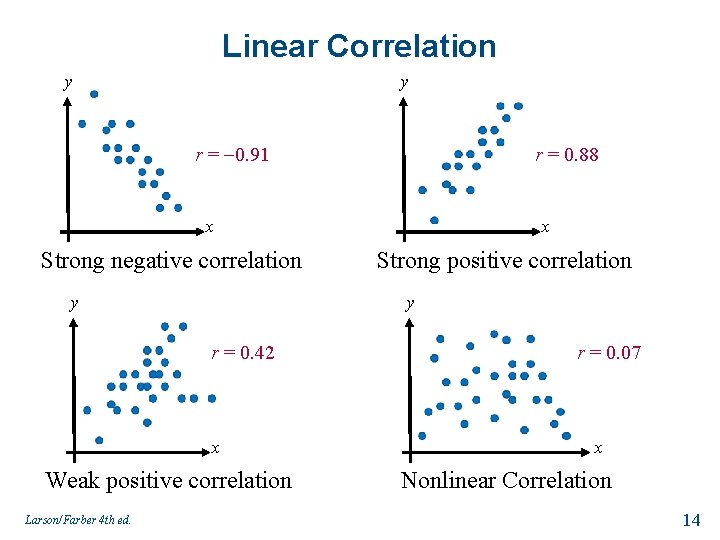
Linear Correlation y y r = 0. 91 r = 0. 88 x Strong negative correlation y Strong positive correlation y r = 0. 42 x Weak positive correlation Larson/Farber 4 th ed. x r = 0. 07 x Nonlinear Correlation 14

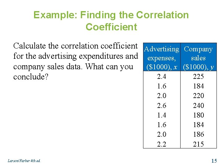
Example: Finding the Correlation Coefficient Calculate the correlation coefficient Advertising Company for the advertising expenditures and expenses, sales company sales data. What can you ($1000), x ($1000), y 2. 4 225 conclude? 1. 6 2. 0 2. 6 1. 4 1. 6 2. 0 2. 2 Larson/Farber 4 th ed. 184 220 240 184 186 215 15

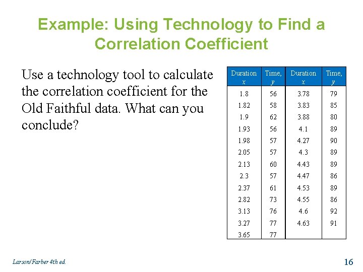
Example: Using Technology to Find a Correlation Coefficient Use a technology tool to calculate the correlation coefficient for the Old Faithful data. What can you conclude? Larson/Farber 4 th ed. Duration x Time, y 1. 8 56 3. 78 79 1. 82 58 3. 83 85 1. 9 62 3. 88 80 1. 93 56 4. 1 89 1. 98 57 4. 27 90 2. 05 57 4. 3 89 2. 13 60 4. 43 89 2. 3 57 4. 47 86 2. 37 61 4. 53 89 2. 82 73 4. 55 86 3. 13 76 4. 6 92 3. 27 77 4. 63 91 3. 65 77 16

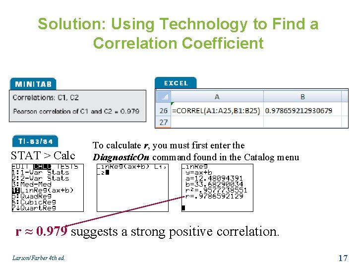
Solution: Using Technology to Find a Correlation Coefficient STAT > Calc To calculate r, you must first enter the Diagnostic. On command found in the Catalog menu r ≈ 0. 979 suggests a strong positive correlation. Larson/Farber 4 th ed. 17

Using a Table to Test a Population Correlation Coefficient ρ • Once the sample correlation coefficient r has been calculated, we need to determine whethere is enough evidence to decide that the population correlation coefficient ρ is significant at a specified level of significance. • Use Table 11 in Appendix B. • If |r| is greater than the critical value, there is enough evidence to decide that the correlation coefficient ρ is significant. Larson/Farber 4 th ed. 18

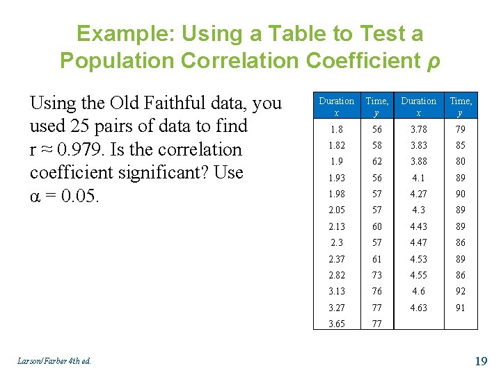
Example: Using a Table to Test a Population Correlation Coefficient ρ Using the Old Faithful data, you used 25 pairs of data to find r ≈ 0. 979. Is the correlation coefficient significant? Use α = 0. 05. Larson/Farber 4 th ed. Duration x Time, y 1. 8 56 3. 78 79 1. 82 58 3. 83 85 1. 9 62 3. 88 80 1. 93 56 4. 1 89 1. 98 57 4. 27 90 2. 05 57 4. 3 89 2. 13 60 4. 43 89 2. 3 57 4. 47 86 2. 37 61 4. 53 89 2. 82 73 4. 55 86 3. 13 76 4. 6 92 3. 27 77 4. 63 91 3. 65 77 19

Correlation and Causation • The fact that two variables are strongly correlated does not in itself imply a cause-and-effect relationship between the variables. • If there is a significant correlation between two variables, you should consider the following possibilities. 1. Is there a direct cause-and-effect relationship between the variables? • Does x cause y? Larson/Farber 4 th ed. 20

Correlation and Causation 2. Is there a reverse cause-and-effect relationship between the variables? • Does y cause x? 3. Is it possible that the relationship between the variables can be caused by a third variable or by a combination of several other variables? 4. Is it possible that the relationship between two variables may be a coincidence? Larson/Farber 4 th ed. 21

Section 9. 2 Linear Regression Larson/Farber 4 th ed. 22

Section 9. 2 Objectives • Find the equation of a regression line • Predict y-values using a regression equation Larson/Farber 4 th ed. 23

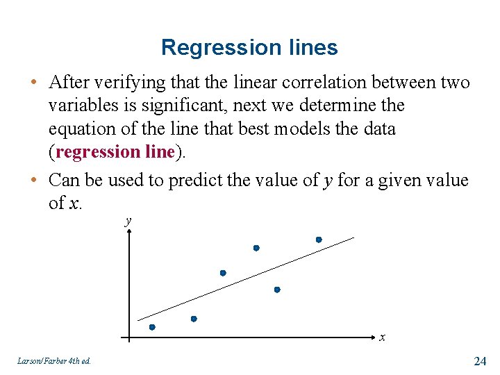
Regression lines • After verifying that the linear correlation between two variables is significant, next we determine the equation of the line that best models the data (regression line). • Can be used to predict the value of y for a given value of x. y x Larson/Farber 4 th ed. 24

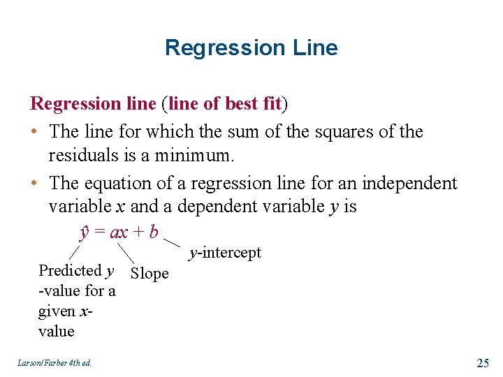
Regression Line Regression line (line of best fit) • The line for which the sum of the squares of the residuals is a minimum. • The equation of a regression line for an independent variable x and a dependent variable y is ŷ = ax + b Predicted y Slope -value for a given xvalue Larson/Farber 4 th ed. y-intercept 25

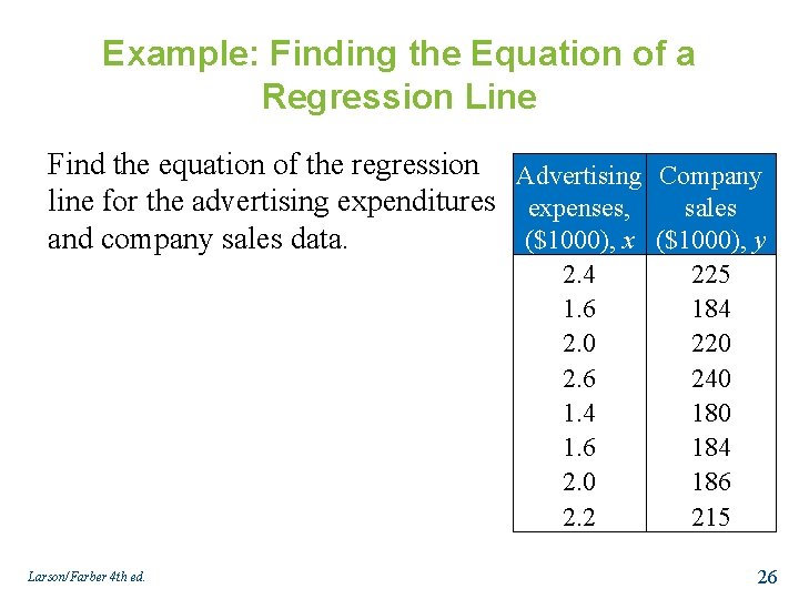
Example: Finding the Equation of a Regression Line Find the equation of the regression Advertising Company line for the advertising expenditures expenses, sales ($1000), x ($1000), y and company sales data. 2. 4 1. 6 2. 0 2. 6 1. 4 1. 6 2. 0 2. 2 Larson/Farber 4 th ed. 225 184 220 240 184 186 215 26

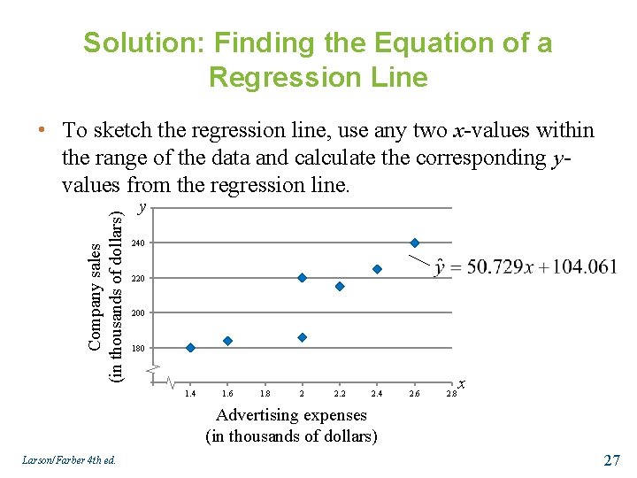
Solution: Finding the Equation of a Regression Line Company sales (in thousands of dollars) • To sketch the regression line, use any two x-values within the range of the data and calculate the corresponding yvalues from the regression line. y 260 240 220 200 180 160 1. 2 1. 4 1. 6 1. 8 2 2. 4 2. 6 2. 8 x Advertising expenses (in thousands of dollars) Larson/Farber 4 th ed. 27

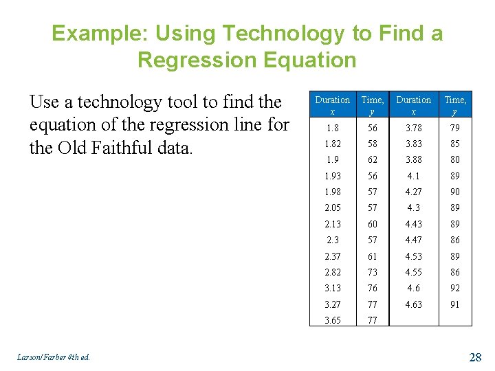
Example: Using Technology to Find a Regression Equation Use a technology tool to find the equation of the regression line for the Old Faithful data. Larson/Farber 4 th ed. Duration x Time, y 1. 8 56 3. 78 79 1. 82 58 3. 83 85 1. 9 62 3. 88 80 1. 93 56 4. 1 89 1. 98 57 4. 27 90 2. 05 57 4. 3 89 2. 13 60 4. 43 89 2. 3 57 4. 47 86 2. 37 61 4. 53 89 2. 82 73 4. 55 86 3. 13 76 4. 6 92 3. 27 77 4. 63 91 3. 65 77 28

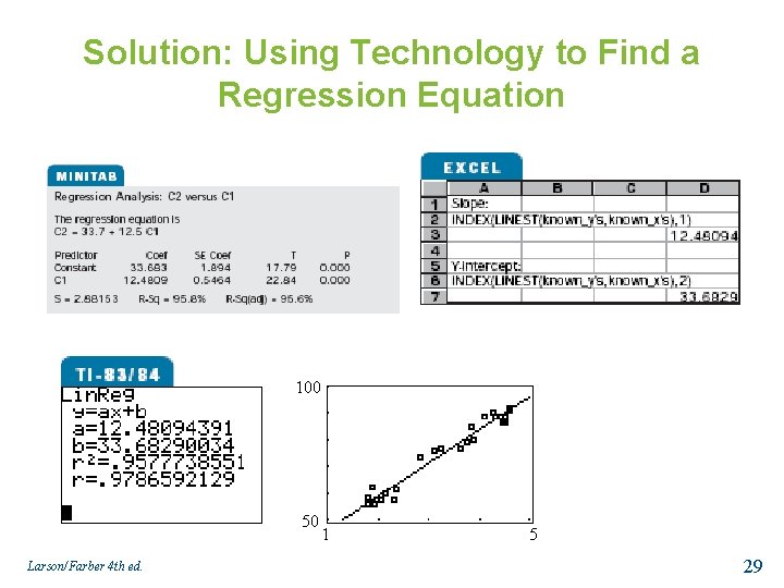
Solution: Using Technology to Find a Regression Equation 100 50 Larson/Farber 4 th ed. 1 5 29

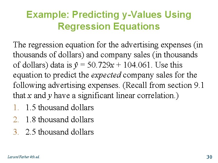
Example: Predicting y-Values Using Regression Equations The regression equation for the advertising expenses (in thousands of dollars) and company sales (in thousands of dollars) data is ŷ = 50. 729 x + 104. 061. Use this equation to predict the expected company sales for the following advertising expenses. (Recall from section 9. 1 that x and y have a significant linear correlation. ) 1. 1. 5 thousand dollars 2. 1. 8 thousand dollars 3. 2. 5 thousand dollars Larson/Farber 4 th ed. 30

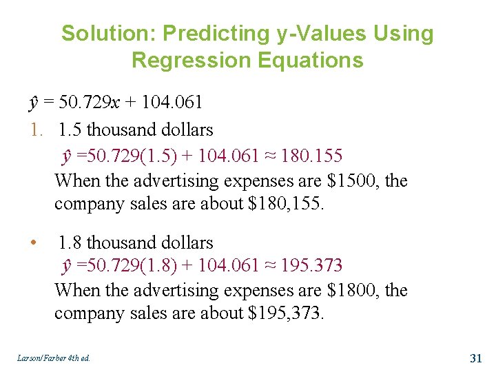
Solution: Predicting y-Values Using Regression Equations ŷ = 50. 729 x + 104. 061 1. 1. 5 thousand dollars ŷ =50. 729(1. 5) + 104. 061 ≈ 180. 155 When the advertising expenses are $1500, the company sales are about $180, 155. • 1. 8 thousand dollars ŷ =50. 729(1. 8) + 104. 061 ≈ 195. 373 When the advertising expenses are $1800, the company sales are about $195, 373. Larson/Farber 4 th ed. 31

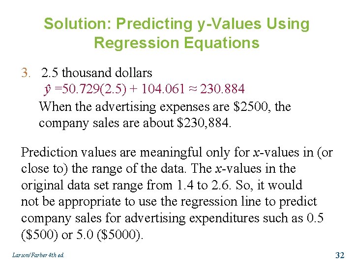
Solution: Predicting y-Values Using Regression Equations 3. 2. 5 thousand dollars ŷ =50. 729(2. 5) + 104. 061 ≈ 230. 884 When the advertising expenses are $2500, the company sales are about $230, 884. Prediction values are meaningful only for x-values in (or close to) the range of the data. The x-values in the original data set range from 1. 4 to 2. 6. So, it would not be appropriate to use the regression line to predict company sales for advertising expenditures such as 0. 5 ($500) or 5. 0 ($5000). Larson/Farber 4 th ed. 32