Chapter 9 Correlation and Regression 9 1 Correlation

Chapter 9: Correlation and Regression • 9. 1 Correlation • 9. 2 Linear Regression • 9. 3 Measures of Regression and Prediction Interval Larson/Farber 1

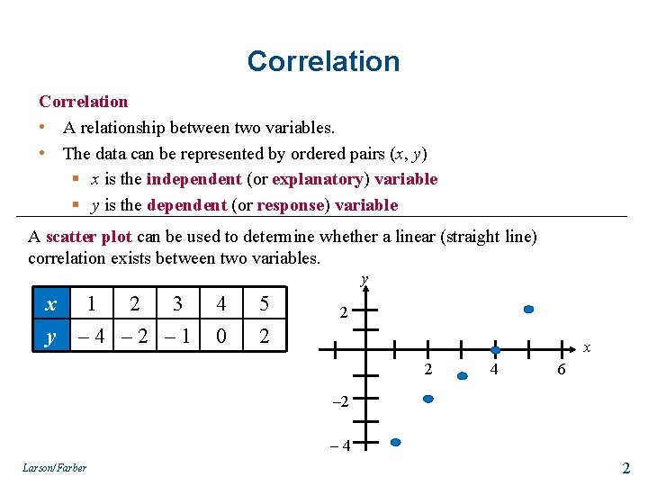
Correlation • A relationship between two variables. • The data can be represented by ordered pairs (x, y) § x is the independent (or explanatory) variable § y is the dependent (or response) variable A scatter plot can be used to determine whether a linear (straight line) correlation exists between two variables. y x y 1 2 3 – 4 – 2 – 1 4 0 5 2 2 x 2 4 6 – 2 – 4 Larson/Farber 2

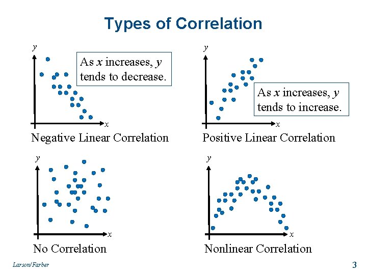
Types of Correlation y y As x increases, y tends to decrease. As x increases, y tends to increase. x x Negative Linear Correlation y y x No Correlation Larson/Farber Positive Linear Correlation x Nonlinear Correlation 3

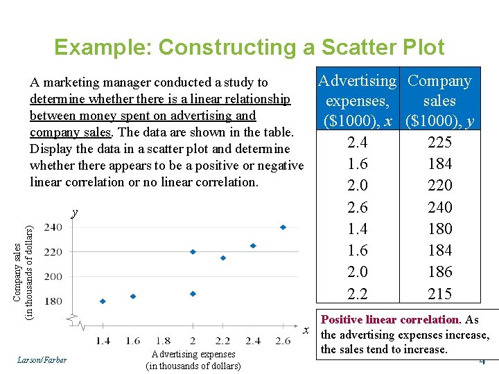
Example: Constructing a Scatter Plot A marketing manager conducted a study to determine whethere is a linear relationship between money spent on advertising and company sales. The data are shown in the table. Display the data in a scatter plot and determine whethere appears to be a positive or negative linear correlation or no linear correlation. Company sales (in thousands of dollars) y Larson/Farber Advertising expenses (in thousands of dollars) Advertising Company expenses, sales ($1000), x ($1000), y 2. 4 225 1. 6 184 2. 0 220 2. 6 240 1. 4 180 1. 6 184 2. 0 186 2. 2 215 Positive linear correlation. As x the advertising expenses increase, the sales tend to increase. 4

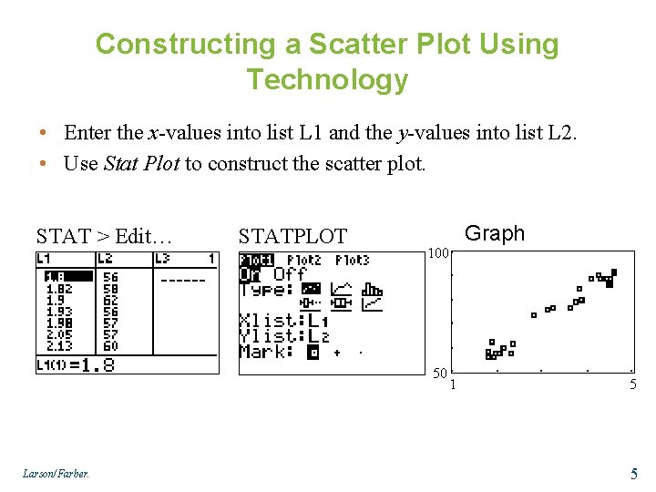
Constructing a Scatter Plot Using Technology • Enter the x-values into list L 1 and the y-values into list L 2. • Use Stat Plot to construct the scatter plot. STAT > Edit… STATPLOT 100 50 Larson/Farber. Graph 1 5 5

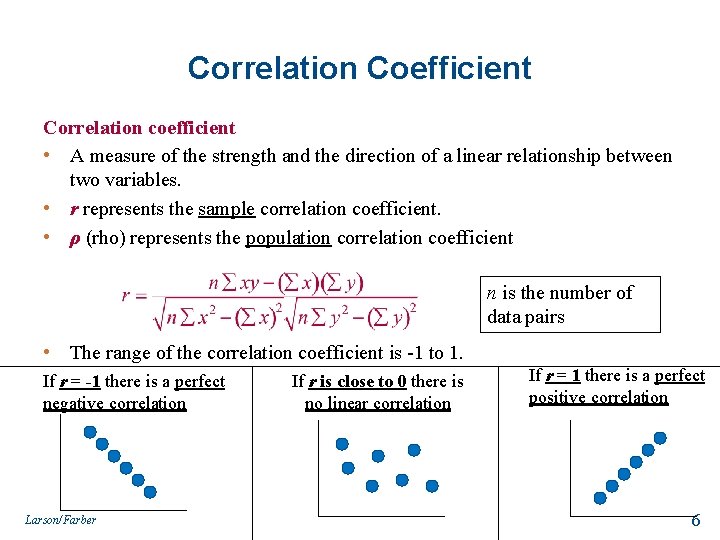
Correlation Coefficient Correlation coefficient • A measure of the strength and the direction of a linear relationship between two variables. • r represents the sample correlation coefficient. • ρ (rho) represents the population correlation coefficient n is the number of data pairs • The range of the correlation coefficient is -1 to 1. If r = -1 there is a perfect negative correlation Larson/Farber If r is close to 0 there is no linear correlation If r = 1 there is a perfect positive correlation 6

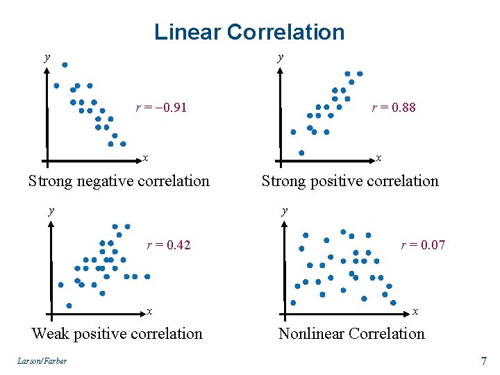
Linear Correlation y y r = 0. 91 r = 0. 88 x Strong negative correlation y Strong positive correlation y r = 0. 42 x Weak positive correlation Larson/Farber x r = 0. 07 x Nonlinear Correlation 7

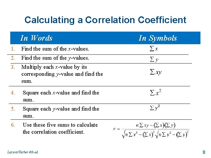
Calculating a Correlation Coefficient In Words 1. Find the sum of the x-values. 2. Find the sum of the y-values. 3. Multiply each x-value by its corresponding y-value and find the sum. 4. Square each x-value and find the sum. 5. Square each y-value and find the sum. 6. Use these five sums to calculate the correlation coefficient. Larson/Farber 4 th ed. In Symbols 8

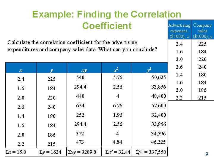
Example: Finding the Correlation Advertising Company Coefficient expenses, sales Calculate the correlation coefficient for the advertising expenditures and company sales data. What can you conclude? x y 225 xy 540 x 2 5. 76 2. 4 1. 6 184 294. 4 2. 56 33, 856 2. 0 220 440 4 48, 400 2. 6 240 624 6. 76 57, 600 1. 4 180 252 1. 96 32, 400 1. 6 184 294. 4 2. 56 33, 856 2. 0 186 372 4 34, 596 2. 2 215 473 4. 84 46, 225 Σx = 15. 8 4 th ed. Σy = 1634 Larson/Farber Σxy = 3289. 8 y 2 50, 625 Σx 2 = 32. 44 Σy 2 = 337, 558 ($1000), x ($1000), y 2. 4 1. 6 2. 0 2. 6 1. 4 1. 6 2. 0 2. 2 225 184 220 240 184 186 215 9

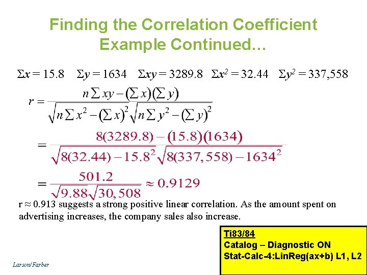
Finding the Correlation Coefficient Example Continued… Σx = 15. 8 Σy = 1634 Σxy = 3289. 8 Σx 2 = 32. 44 Σy 2 = 337, 558 r ≈ 0. 913 suggests a strong positive linear correlation. As the amount spent on advertising increases, the company sales also increase. Larson/Farber Ti 83/84 Catalog – Diagnostic ON Stat-Calc-4: Lin. Reg(ax+b) L 1, L 2 10

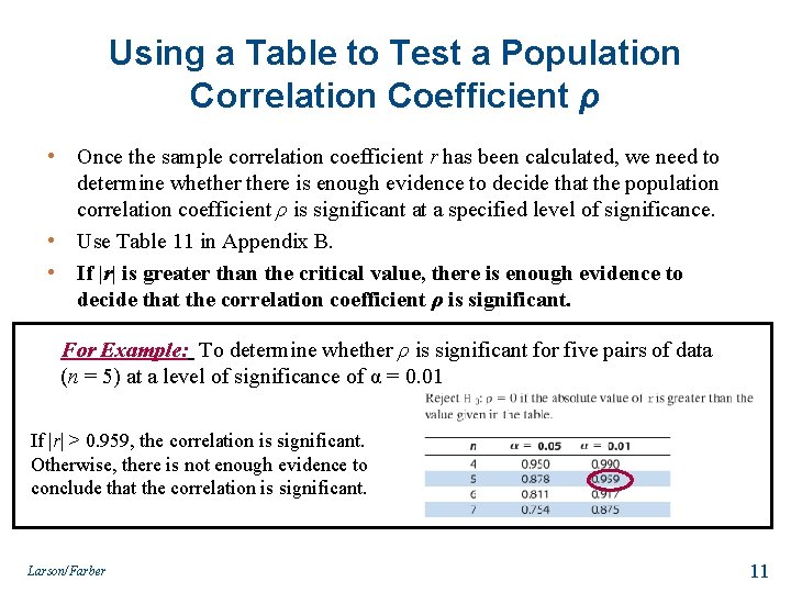
Using a Table to Test a Population Correlation Coefficient ρ • Once the sample correlation coefficient r has been calculated, we need to determine whethere is enough evidence to decide that the population correlation coefficient ρ is significant at a specified level of significance. • Use Table 11 in Appendix B. • If |r| is greater than the critical value, there is enough evidence to decide that the correlation coefficient ρ is significant. For Example: To determine whether ρ is significant for five pairs of data (n = 5) at a level of significance of α = 0. 01 If |r| > 0. 959, the correlation is significant. Otherwise, there is not enough evidence to conclude that the correlation is significant. Larson/Farber 11

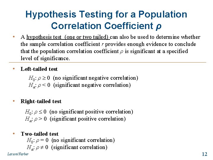
Hypothesis Testing for a Population Correlation Coefficient ρ • A hypothesis test (one or two tailed) can also be used to determine whether the sample correlation coefficient r provides enough evidence to conclude that the population correlation coefficient ρ is significant at a specified level of significance. • Left-tailed test H 0: ρ 0 (no significant negative correlation) Ha: ρ < 0 (significant negative correlation) • Right-tailed test H 0: ρ 0 (no significant positive correlation) Ha: ρ > 0 (significant positive correlation) • Two-tailed test H 0: ρ = 0 (no significant correlation) Ha: ρ 0 (significant correlation) Larson/Farber 12

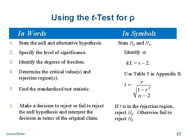
Using the t-Test for ρ In Words In Symbols 1. State the null and alternative hypothesis. 2. Specify the level of significance. Identify . 3. Identify the degrees of freedom. d. f. = n – 2. 4. Determine the critical value(s) and rejection region(s). Use Table 5 in Appendix B. 5. Find the standardized test statistic. 6. Make a decision to reject or fail to reject the null hypothesis and interpret the decision in terms of the original claim. Larson/Farber State H 0 and Ha. If t is in the rejection region, reject H 0. Otherwise fail to reject H 0. 13

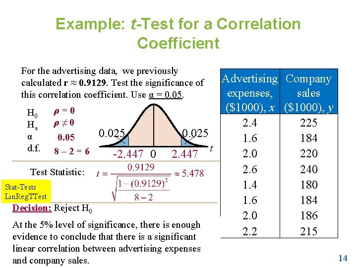
Example: t-Test for a Correlation Coefficient For the advertising data, we previously calculated r ≈ 0. 9129. Test the significance of this correlation coefficient. Use α = 0. 05. Advertising Company expenses, sales ($1000), x ($1000), y ρ=0 H 0 ρ≠ 0 2. 4 225 Ha 0. 025 α 0. 05 1. 6 184 d. f. 8 – 2 = 6 t 2. 0 220 -2. 447 0 2. 447 2. 6 240 Test Statistic: 1. 4 180 Stat-Tests Lin. Reg. TTest 1. 6 184 Decision: Reject H 0 2. 0 186 At the 5% level of significance, there is enough 2. 2 215 evidence to conclude that there is a significant linear correlation between advertising expenses Larson/Farber 4 th ed. and company sales. 14

Correlation and Causation • The fact that two variables are strongly correlated does not in itself imply a cause-and-effect relationship between the variables. • If there is a significant correlation between two variables, you should consider the following possibilities: 1. Is there a direct cause-and-effect relationship between the variables? • Does x cause y? 2. Is there a reverse cause-and-effect relationship between the variables? • Does y cause x? 3. Is it possible that the relationship between the variables can be caused by a third variable or by a combination of several other variables? 4. Is it possible that the relationship between two variables may be a coincidence? Larson/Farber 15

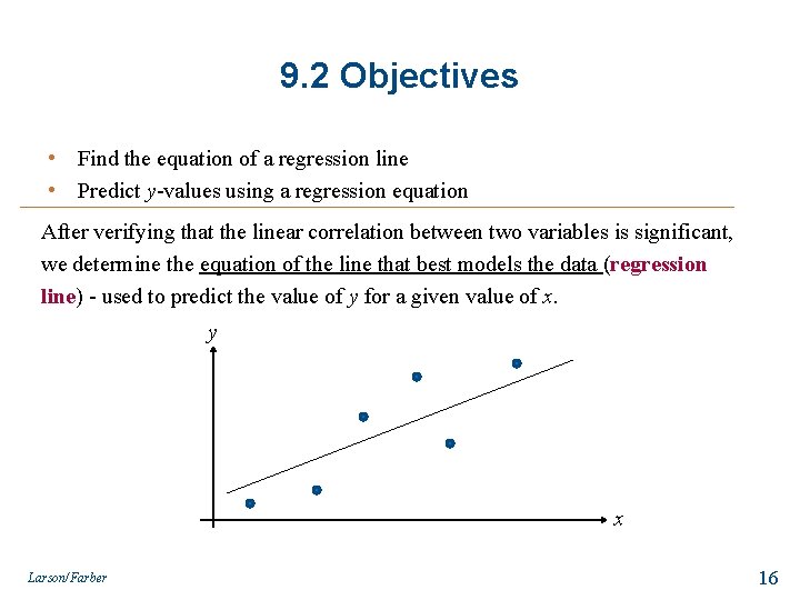
9. 2 Objectives • Find the equation of a regression line • Predict y-values using a regression equation After verifying that the linear correlation between two variables is significant, we determine the equation of the line that best models the data (regression line) - used to predict the value of y for a given value of x. y x Larson/Farber 16

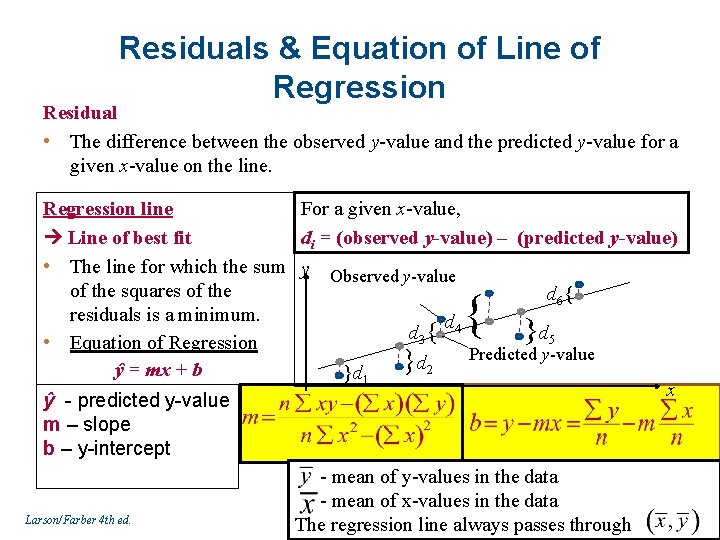
Residuals & Equation of Line of Regression Residual • The difference between the observed y-value and the predicted y-value for a given x-value on the line. Regression line For a given x-value, Line of best fit di = (observed y-value) – (predicted y-value) • The line for which the sum y Observed y-value of the squares of the d 6{ residuals is a minimum. d 4 d 5 d { 3 • Equation of Regression Predicted y-value } d 2 ŷ = mx + b }d 1 x ŷ - predicted y-value m – slope b – y-intercept - mean of y-values in the data - mean of x-values in the data Larson/Farber 4 th ed. 17 The regression line always passes through { }

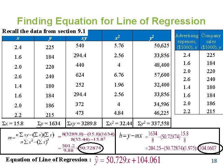
Finding Equation for Line of Regression Recall the data from section 9. 1 x y 225 xy 540 x 2 5. 76 2. 4 1. 6 184 294. 4 2. 56 33, 856 2. 0 220 440 4 48, 400 2. 6 240 624 6. 76 57, 600 1. 4 180 252 1. 96 32, 400 1. 6 184 294. 4 2. 56 33, 856 2. 0 186 372 4 34, 596 2. 2 215 473 4. 84 46, 225 Σx = 15. 8 4 th ed. Σy = 1634 Larson/Farber Σxy = 3289. 8 Equation of Line of Regression : y 2 50, 625 Advertising Company expenses, sales ($1000), x ($1000), y 2. 4 1. 6 2. 0 2. 6 1. 4 1. 6 2. 0 2. 2 225 184 220 240 184 186 215 Σx 2 = 32. 44 Σy 2 = 337, 558 18

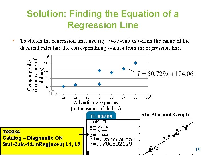
Solution: Finding the Equation of a Regression Line Company sales (in thousands of dollars) • To sketch the regression line, use any two x-values within the range of the data and calculate the corresponding y-values from the regression line. 260 y 240 220 200 180 160 1. 2 1. 4 1. 6 1. 8 2 2. 2 Advertising expenses (in thousands of dollars) Ti 83/84 Catalog – Diagnostic ON Stat-Calc-4: Lin. Reg(ax+b) L 1, L 2 Larson/Farber 4 th ed. 2. 4 2. 6 x 2. 8 Stat. Plot and Graph Ax + b 50. 729 104. 061 19

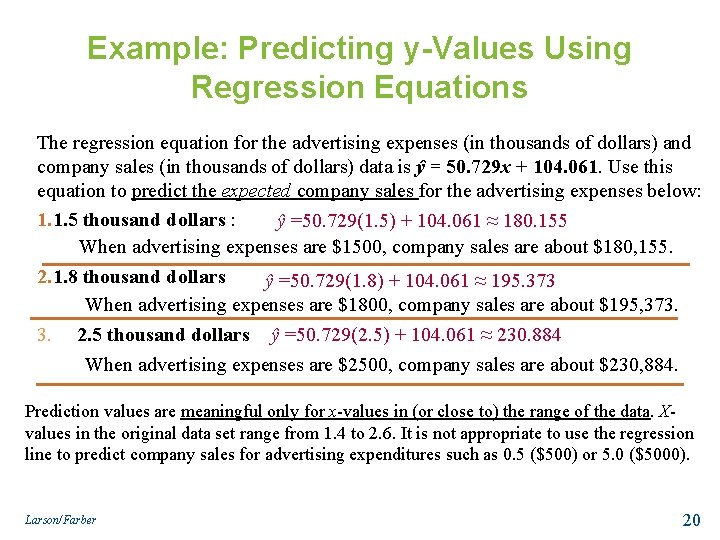
Example: Predicting y-Values Using Regression Equations The regression equation for the advertising expenses (in thousands of dollars) and company sales (in thousands of dollars) data is ŷ = 50. 729 x + 104. 061. Use this equation to predict the expected company sales for the advertising expenses below: 1. 1. 5 thousand dollars : ŷ =50. 729(1. 5) + 104. 061 ≈ 180. 155 When advertising expenses are $1500, company sales are about $180, 155. 2. 1. 8 thousand dollars ŷ =50. 729(1. 8) + 104. 061 ≈ 195. 373 When advertising expenses are $1800, company sales are about $195, 373. 3. 2. 5 thousand dollars ŷ =50. 729(2. 5) + 104. 061 ≈ 230. 884 When advertising expenses are $2500, company sales are about $230, 884. Prediction values are meaningful only for x-values in (or close to) the range of the data. Xvalues in the original data set range from 1. 4 to 2. 6. It is not appropriate to use the regression line to predict company sales for advertising expenditures such as 0. 5 ($500) or 5. 0 ($5000). Larson/Farber 20

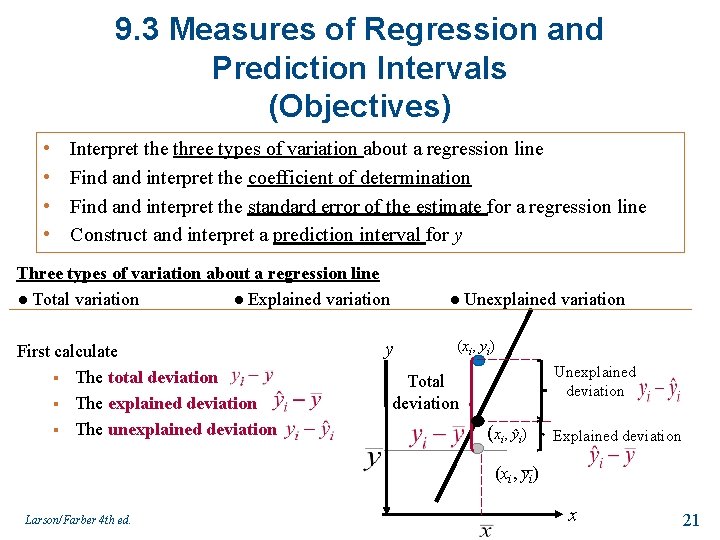
9. 3 Measures of Regression and Prediction Intervals (Objectives) • • Interpret the three types of variation about a regression line Find and interpret the coefficient of determination Find and interpret the standard error of the estimate for a regression line Construct and interpret a prediction interval for y Three types of variation about a regression line ● Total variation ● Explained variation First calculate § The total deviation § The explained deviation § The unexplained deviation ● Unexplained variation y (xi, yi) Unexplained deviation Total deviation (xi, ŷi) Explained deviation (xi, yi) Larson/Farber 4 th ed. x 21

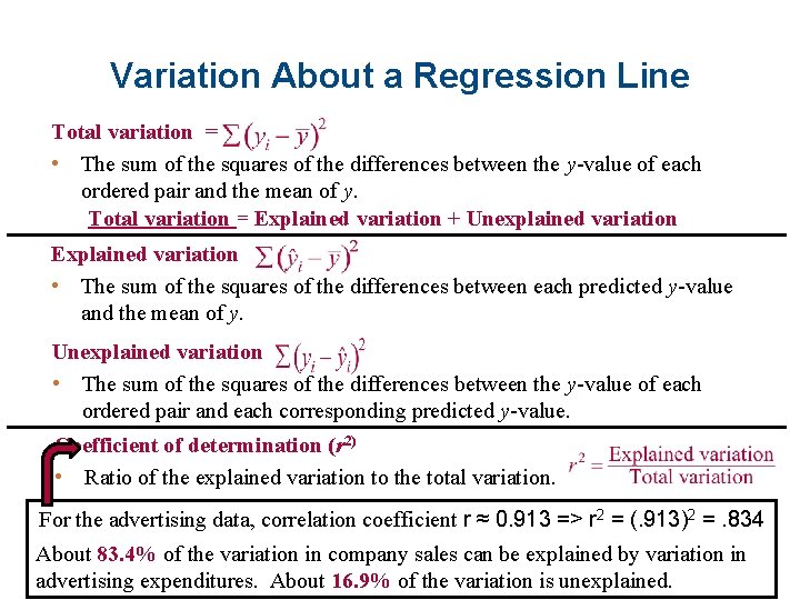
Variation About a Regression Line Total variation = • The sum of the squares of the differences between the y-value of each ordered pair and the mean of y. Total variation = Explained variation + Unexplained variation Explained variation • The sum of the squares of the differences between each predicted y-value and the mean of y. Unexplained variation • The sum of the squares of the differences between the y-value of each ordered pair and each corresponding predicted y-value. Coefficient of determination (r 2) • Ratio of the explained variation to the total variation. For the advertising data, correlation coefficient r ≈ 0. 913 => r 2 = (. 913)2 =. 834 About 83. 4% of the variation in company sales can be explained by variation in Larson/Farber 4 th ed. 22 advertising expenditures. About 16. 9% of the variation is unexplained.

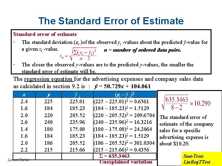
The Standard Error of Estimate Standard error of estimate • The standard deviation (se )of the observed yi -values about the predicted ŷ-value for a given xi -value. n = number of ordered data pairs. • The closer the observed y-values are to the predicted y-values, the smaller the standard error of estimate will be. The regression equation for the advertising expenses and company sales data as calculated in section 9. 2 is : ŷ = 50. 729 x + 104. 061 x 2. 4 1. 6 2. 0 2. 6 1. 4 1. 6 2. 0 2. 2 Larson/Farber y 225 184 220 240 184 186 215 ŷi 225. 81 185. 23 205. 52 235. 96 175. 08 185. 23 205. 52 215. 66 (yi – ŷ i)2 (225 – 225. 81)2 = 0. 6561 (184 – 185. 23)2 = 1. 5129 (220 – 205. 52)2 = 209. 6704 (240 – 235. 96)2 = 16. 3216 (180 – 175. 08)2 = 24. 2064 (184 – 185. 23)2 = 1. 5129 (186 – 205. 52)2 = 381. 0304 (215 – 215. 66)2 = 0. 4356 Σ = 635. 3463 Unexplained variation The standard error of estimate of the company sales for a specific advertising expense is about $10. 29. Stat-Tests Lin. Reg. TTest 23

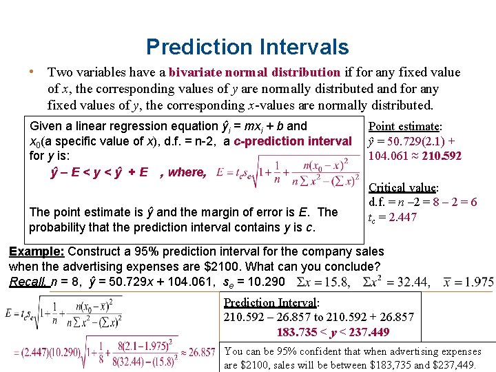
Prediction Intervals • Two variables have a bivariate normal distribution if for any fixed value of x, the corresponding values of y are normally distributed and for any fixed values of y, the corresponding x-values are normally distributed. Given a linear regression equation ŷi = mxi + b and x 0(a specific value of x), d. f. = n-2, a c-prediction interval for y is: ŷ – E < y < ŷ + E , where, The point estimate is ŷ and the margin of error is E. The probability that the prediction interval contains y is c. Point estimate: ŷ = 50. 729(2. 1) + 104. 061 ≈ 210. 592 Critical value: d. f. = n – 2 = 8 – 2 = 6 tc = 2. 447 Example: Construct a 95% prediction interval for the company sales when the advertising expenses are $2100. What can you conclude? Recall, n = 8, ŷ = 50. 729 x + 104. 061, se = 10. 290 Prediction Interval: 210. 592 – 26. 857 to 210. 592 + 26. 857 183. 735 < y < 237. 449 Larson/Farber 4 th ed. You can be 95% confident that when advertising expenses 24 are $2100, sales will be between $183, 735 and $237, 449.