Chapter 9 Classification and Clustering Classification and Clustering

Chapter 9 Classification and Clustering

Classification and Clustering n n n Classification/clustering are classical pattern recognition/ machine learning problems Classification, also referred to as categorization Ø Asks “what class does this item belong to? ” Ø Supervised learning task Clustering Ø Asks “how can I group this set of items? ” Ø Unsupervised learning task n Items can be documents, emails, queries, entities, images n Useful for a wide variety of search engine tasks 2

Classification n Classification is the task of automatically applying labels to items Useful for many search-related tasks Ø Spam detection Ø Sentiment classification Ø Online advertising Two common approaches Ø Probabilistic Ø Geometric 3

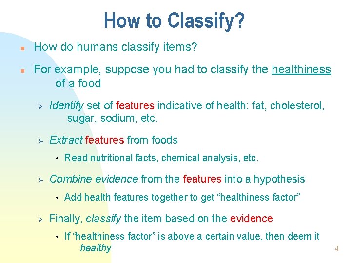
How to Classify? n n How do humans classify items? For example, suppose you had to classify the healthiness of a food Ø Ø Identify set of features indicative of health: fat, cholesterol, sugar, sodium, etc. Extract features from foods • Ø Combine evidence from the features into a hypothesis • Ø Read nutritional facts, chemical analysis, etc. Add health features together to get “healthiness factor” Finally, classify the item based on the evidence • If “healthiness factor” is above a certain value, then deem it healthy 4

Ontologies n Ontology is a labeling or categorization scheme n Examples n Ø Binary (spam, not spam) Ø Multi-valued (red, green, blue) Ø Hierarchical (news/local/sports) Different classification tasks require different ontologies 5

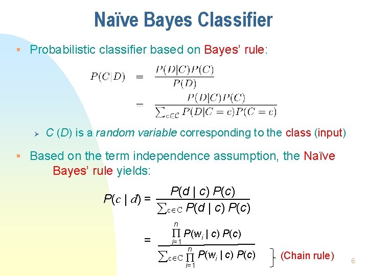
Naïve Bayes Classifier § Probabilistic classifier based on Bayes’ rule: Ø C (D) is a random variable corresponding to the class (input) § Based on the term independence assumption, the Naïve Bayes’ rule yields: P(d | c) P(c | d) = c C P(d | c) P(c) n = P(wi | c) P(c) i=1 n c C P(wi | c) P(c) i=1 (Chain rule) 6

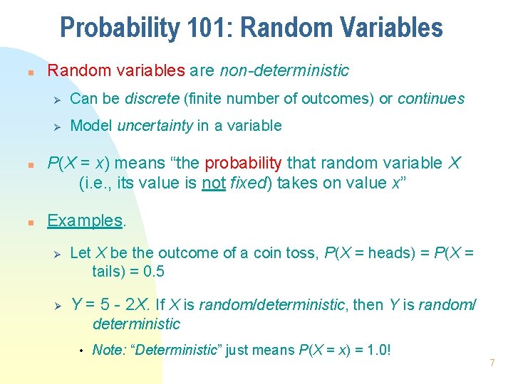
Probability 101: Random Variables n n n Random variables are non-deterministic Ø Can be discrete (finite number of outcomes) or continues Ø Model uncertainty in a variable P(X = x) means “the probability that random variable X (i. e. , its value is not fixed) takes on value x” Examples. Ø Ø Let X be the outcome of a coin toss, P(X = heads) = P(X = tails) = 0. 5 Y = 5 - 2 X. If X is random/deterministic, then Y is random/ deterministic • Note: “Deterministic” just means P(X = x) = 1. 0! 7

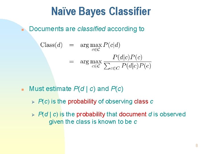
Naïve Bayes Classifier n Documents are classified according to n Must estimate P(d | c) and P(c) Ø Ø P(c) is the probability of observing class c P(d | c) is the probability that document d is observed given the class is known to be c 8

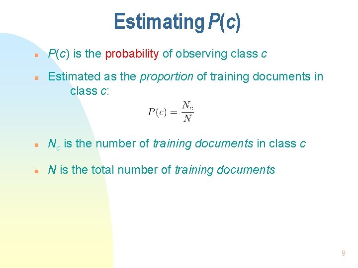
Estimating P(c) n n P(c) is the probability of observing class c Estimated as the proportion of training documents in class c: n Nc is the number of training documents in class c n N is the total number of training documents 9

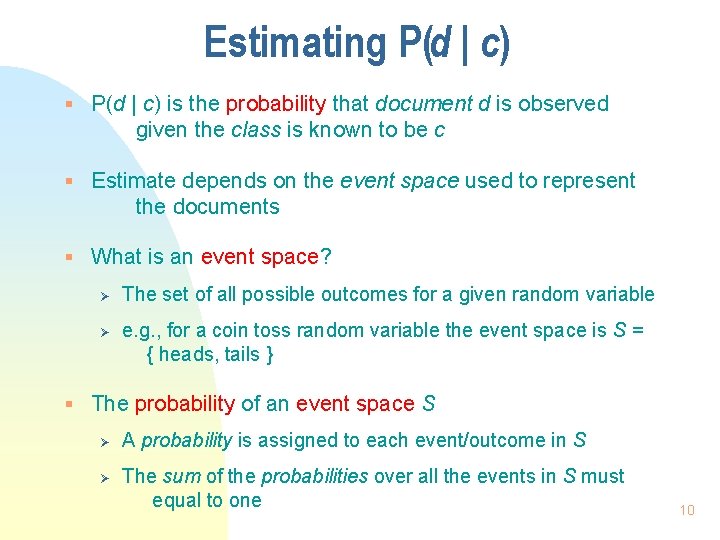
Estimating P(d | c) § P(d | c) is the probability that document d is observed given the class is known to be c § Estimate depends on the event space used to represent the documents § What is an event space? Ø Ø The set of all possible outcomes for a given random variable e. g. , for a coin toss random variable the event space is S = { heads, tails } § The probability of an event space S Ø Ø A probability is assigned to each event/outcome in S The sum of the probabilities over all the events in S must equal to one 10

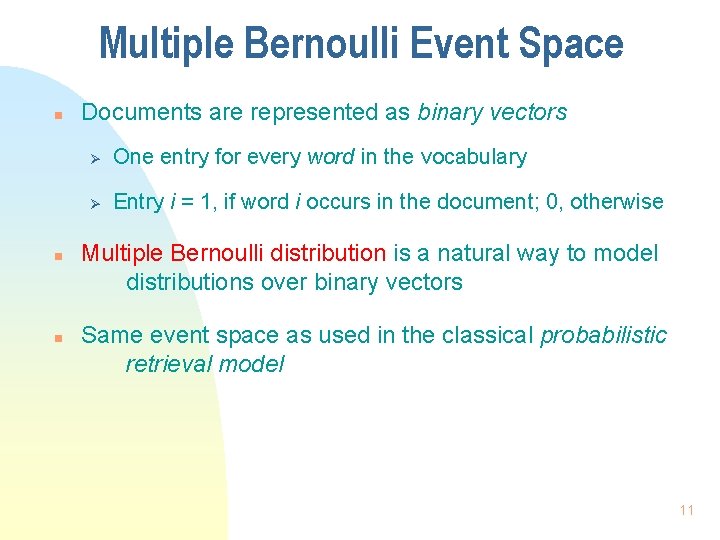
Multiple Bernoulli Event Space n n n Documents are represented as binary vectors Ø One entry for every word in the vocabulary Ø Entry i = 1, if word i occurs in the document; 0, otherwise Multiple Bernoulli distribution is a natural way to model distributions over binary vectors Same event space as used in the classical probabilistic retrieval model 11

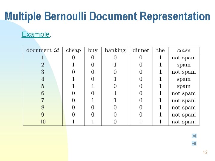
Multiple Bernoulli Document Representation Example. 12

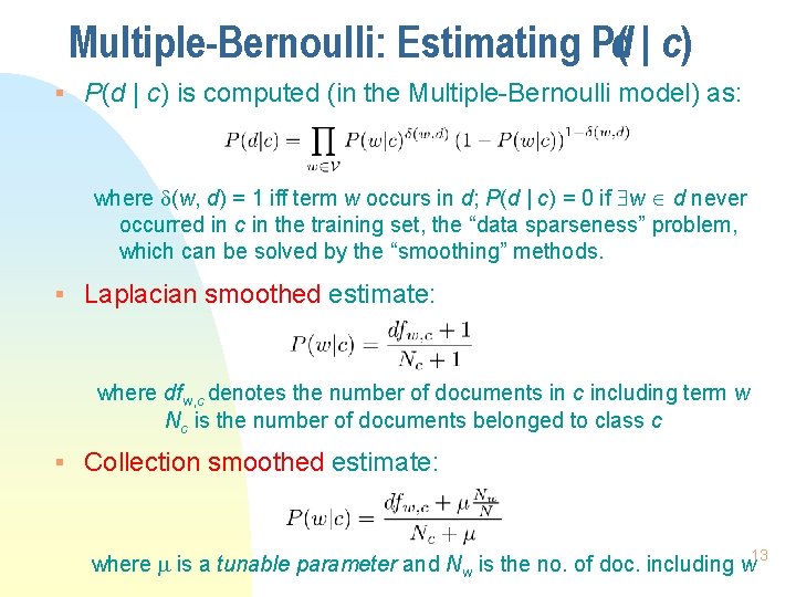
Multiple-Bernoulli: Estimating P(d | c) § P(d | c) is computed (in the Multiple-Bernoulli model) as: where (w, d) = 1 iff term w occurs in d; P(d | c) = 0 if w d never occurred in c in the training set, the “data sparseness” problem, which can be solved by the “smoothing” methods. § Laplacian smoothed estimate: where dfw, c denotes the number of documents in c including term w Nc is the number of documents belonged to class c § Collection smoothed estimate: where is a tunable parameter and Nw is the no. of doc. including w 13

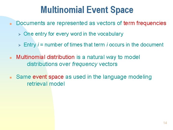
Multinomial Event Space n n n Documents are represented as vectors of term frequencies Ø One entry for every word in the vocabulary Ø Entry i = number of times that term i occurs in the document Multinomial distribution is a natural way to model distributions over frequency vectors Same event space as used in the language modeling retrieval model 14

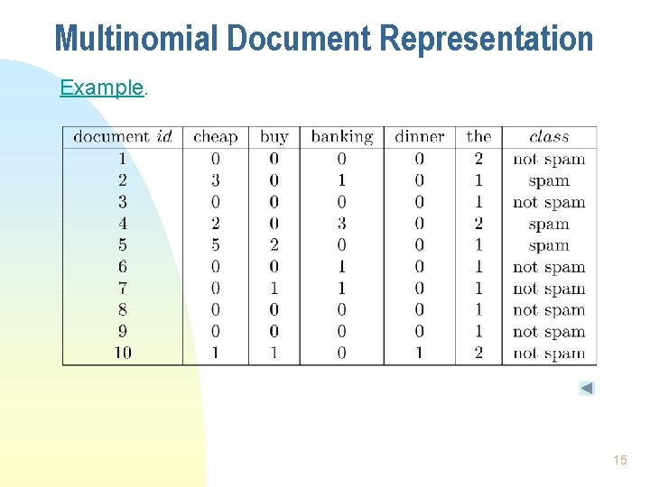
Multinomial Document Representation Example. 15

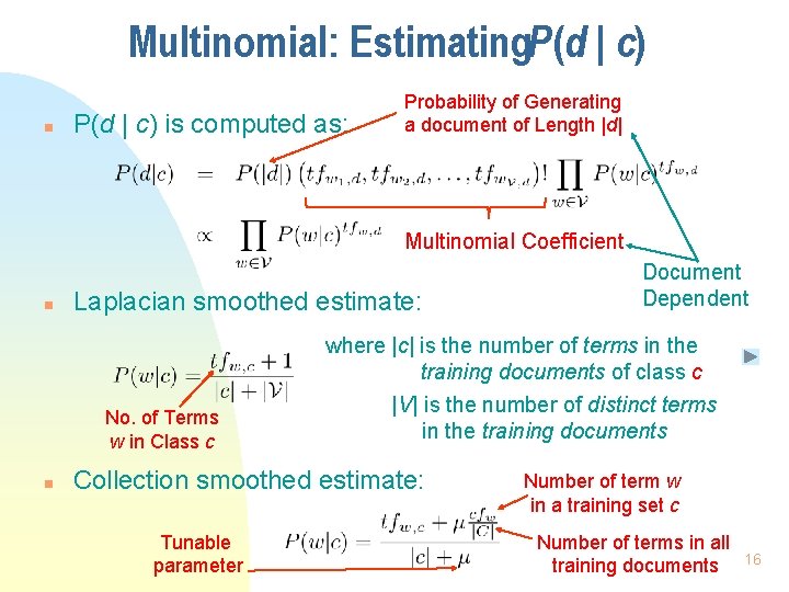
Multinomial: Estimating. P(d | c) n P(d | c) is computed as: Probability of Generating a document of Length |d| Multinomial Coefficient n Laplacian smoothed estimate: No. of Terms w in Class c n where |c| is the number of terms in the training documents of class c |V| is the number of distinct terms in the training documents Collection smoothed estimate: Tunable parameter Document Dependent Number of term w in a training set c Number of terms in all training documents 16

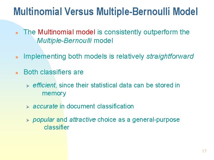
Multinomial Versus Multiple-Bernoulli Model n The Multinomial model is consistently outperform the Multiple-Bernoulli model n Implementing both models is relatively straightforward n Both classifiers are Ø Ø Ø efficient, since their statistical data can be stored in memory accurate in document classification popular and attractive choice as a general-purpose classifier 17

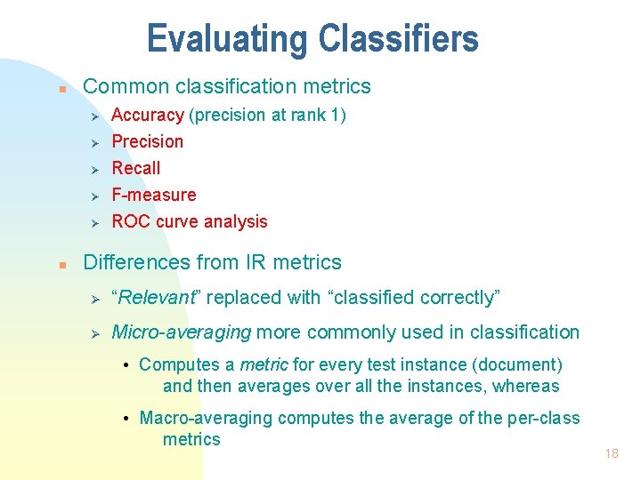
Evaluating Classifiers n Common classification metrics Ø Ø Ø n Accuracy (precision at rank 1) Precision Recall F-measure ROC curve analysis Differences from IR metrics Ø “Relevant” replaced with “classified correctly” Ø Micro-averaging more commonly used in classification • Computes a metric for every test instance (document) and then averages over all the instances, whereas • Macro-averaging computes the average of the per-class metrics 18

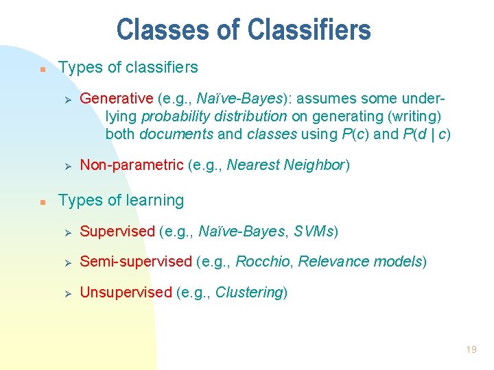
Classes of Classifiers n Types of classifiers Ø Ø n Generative (e. g. , Naïve-Bayes): assumes some underlying probability distribution on generating (writing) both documents and classes using P(c) and P(d | c) Non-parametric (e. g. , Nearest Neighbor) Types of learning Ø Supervised (e. g. , Naïve-Bayes, SVMs) Ø Semi-supervised (e. g. , Rocchio, Relevance models) Ø Unsupervised (e. g. , Clustering) 19

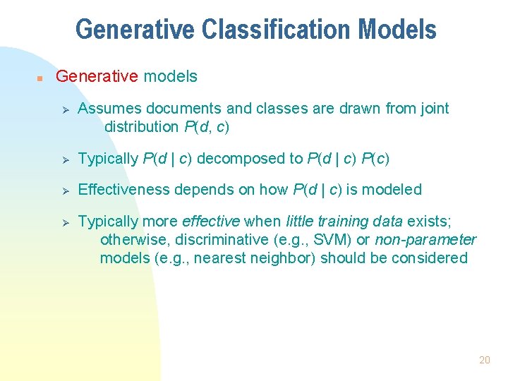
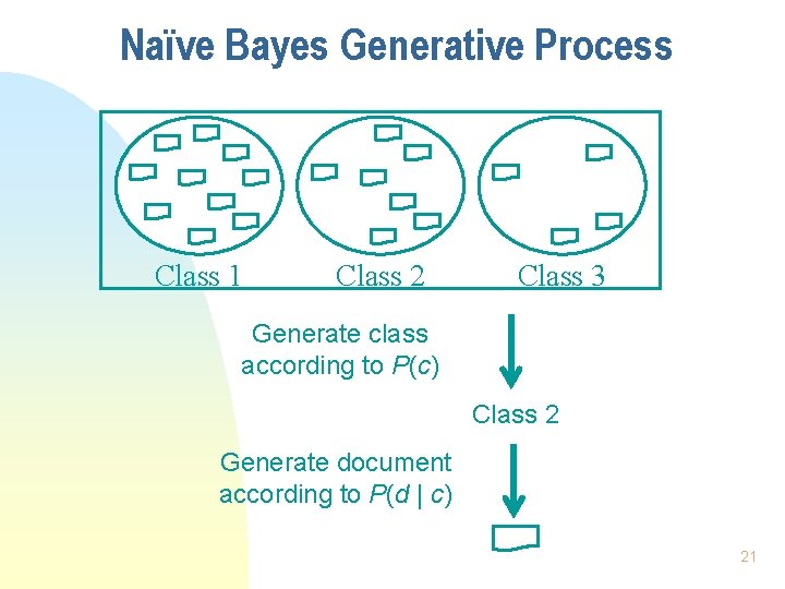
Generative Classification Models n Generative models Ø Assumes documents and classes are drawn from joint distribution P(d, c) Ø Typically P(d | c) decomposed to P(d | c) P(c) Ø Effectiveness depends on how P(d | c) is modeled Ø Typically more effective when little training data exists; otherwise, discriminative (e. g. , SVM) or non-parameter models (e. g. , nearest neighbor) should be considered 20

Naïve Bayes Generative Process Class 1 Class 2 Class 3 Generate class according to P(c) Class 2 Generate document according to P(d | c) 21

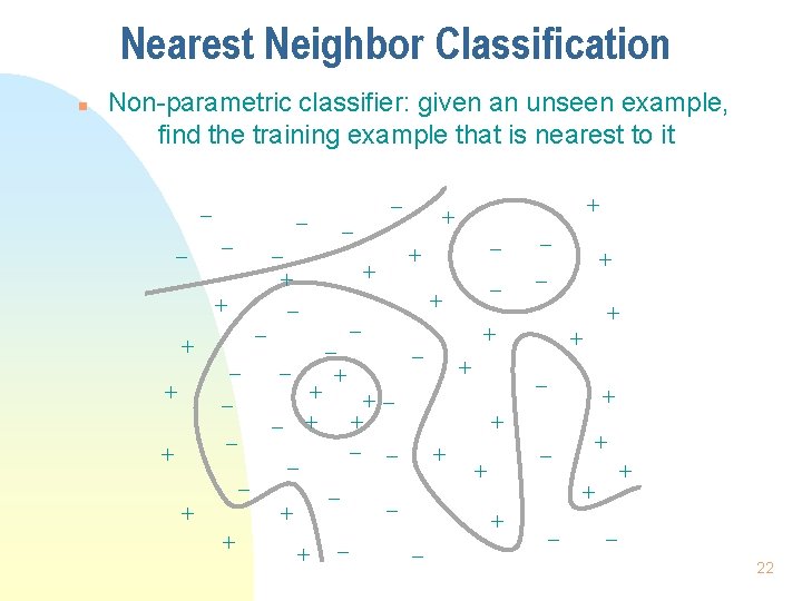
Nearest Neighbor Classification n Non-parametric classifier: given an unseen example, find the training example that is nearest to it – – – – + + + – + – – – – + + + – + + + – +– + – – – + + + – – + + – – – 22

Feature Selection n Document classifiers can have a very large number of features Ø Ø n Not all features are useful Excessive features can increase computational cost of training and testing Feature selection methods reduce the number of features by choosing the most useful features Ø which can significantly improve efficiency (in terms of storage and processing time) while not hurting the effectiveness much (in addition to eliminating noisy) 23

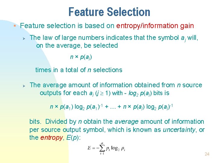
Feature Selection § Feature selection is based on entropy/information gain Ø The law of large numbers indicates that the symbol aj will, on the average, be selected n × p(aj) times in a total of n selections Ø The average amount of information obtained from n source outputs for each aj (j 1) with - log 2 p(aj) bits is n × p(a 1) log 2 p(a 1)-1 + + n × p(aj) log 2 p(aj)-1 bits. Divided by n obtain the average amount of information per source output symbol, which is known as uncertainty, or the entropy, E(p): 24

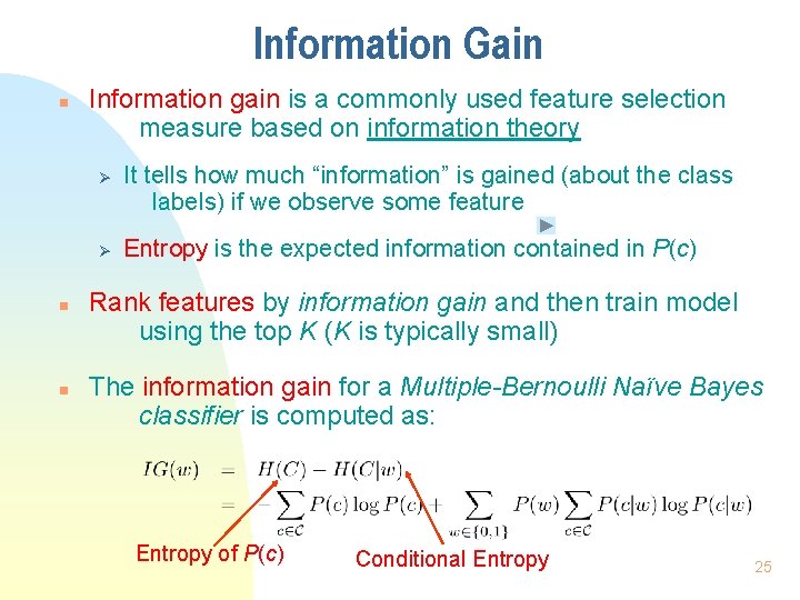
Information Gain n Information gain is a commonly used feature selection measure based on information theory Ø Ø n n It tells how much “information” is gained (about the class labels) if we observe some feature Entropy is the expected information contained in P(c) Rank features by information gain and then train model using the top K (K is typically small) The information gain for a Multiple-Bernoulli Naïve Bayes classifier is computed as: Entropy of P(c) Conditional Entropy 25

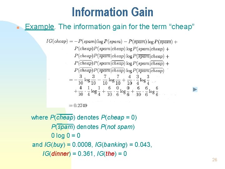
Information Gain n Example. The information gain for the term “cheap” where P(cheap) denotes P(cheap = 0) P(spam) denotes P(not spam) 0 log 0 = 0 and IG(buy) = 0. 0008, IG(banking) = 0. 043, IG(dinner) = 0. 361, IG(the) = 0 26

Classification Applications n Classification is widely used to enhance search engines n Example applications Ø Spam detection Ø Sentiment classification Ø Ø Semantic classification of advertisements (based on the semantically-related, not topically-related scope) Others … 27

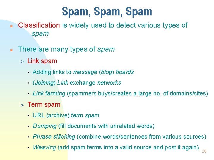
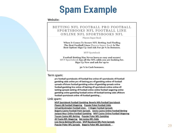
Spam, Spam n n Classification is widely used to detect various types of spam There are many types of spam Ø Ø Link spam • Adding links to message (blog) boards • (Joining) Link exchange networks • Link farming (spammers buys/creates a large no. of domains/sites) Term spam • URL (archive) term spam • Dumping (fill documents with unrelated words) • Phrase stitching (combine words/sentences from various sources) • Weaving (add spam terms into a valid source and post it again) 28

Spam Example 29

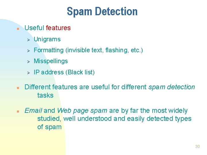
Spam Detection n Useful features Ø Unigrams Ø Formatting (invisible text, flashing, etc. ) Ø Misspellings Ø IP address (Black list) Different features are useful for different spam detection tasks Email and Web page spam are by far the most widely studied, well understood and easily detected types of spam 30

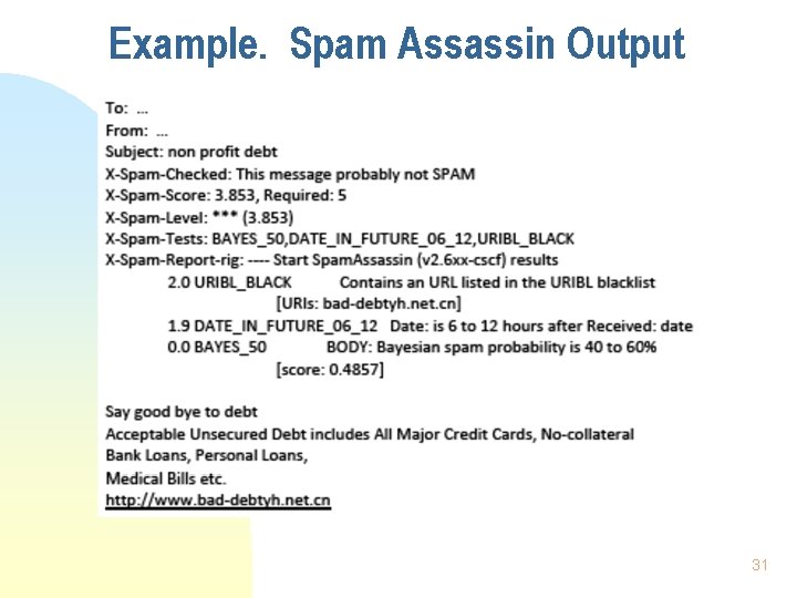
Example. Spam Assassin Output 31

Sentiment n n n Blogs, online reviews/forum posts are often opinionated Sentiment classification attempts to automatically identify the polarity of the opinion Ø Negative opinion Ø Neutral opinion Ø Positive opinion Sometimes the strength of the opinion is also important Ø “Two stars” vs. “four stars” Ø Weakly negative vs. strongly negative 32

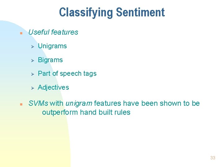
Classifying Sentiment n n Useful features Ø Unigrams Ø Bigrams Ø Part of speech tags Ø Adjectives SVMs with unigram features have been shown to be outperform hand built rules 33

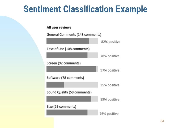
Sentiment Classification Example 34

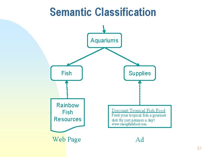
Classifying Online Ads n n Unlike traditional search, online advertising goes beyond “topical relevance” A user searching for ‘tropical fish’ may also be interested in pet stores, local aquariums, or even scuba diving lessons These are semantically related, but not topically relevant! We can bridge the semantic gap by classifying ads and queries according to a semantic hierarchy 35

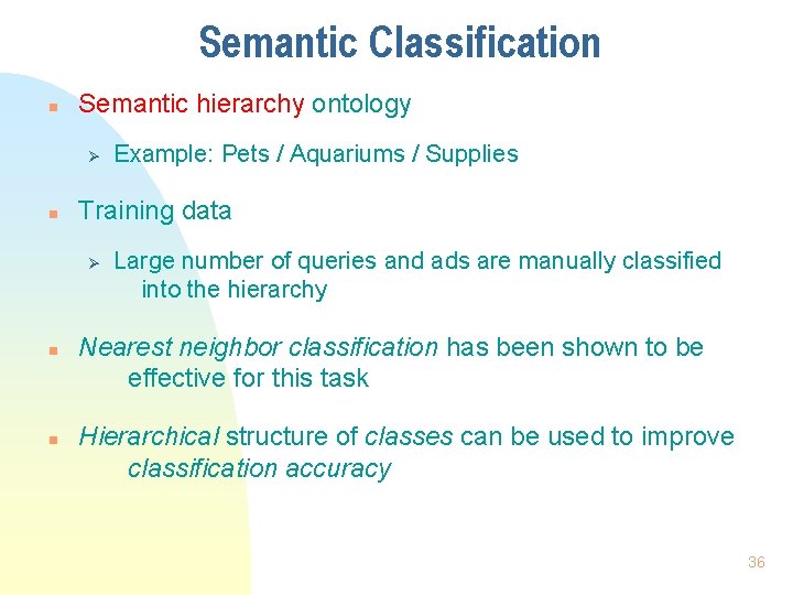
Semantic Classification n Semantic hierarchy ontology Ø n Training data Ø n n Example: Pets / Aquariums / Supplies Large number of queries and ads are manually classified into the hierarchy Nearest neighbor classification has been shown to be effective for this task Hierarchical structure of classes can be used to improve classification accuracy 36

Semantic Classification Aquariums Fish Supplies Rainbow Fish Resources Discount Tropical Fish Food Web Page Ad Feed your tropical fish a gourmet diet for just pennies a day! www. cheapfishfood. com 37

Clustering n n A set of unsupervised algorithms that attempt to find latent structure in a set of items Goal is to identify groups (clusters) of similar items, given a set of unlabeled instances Suppose I gave you the shape, color, vitamin C content and price of various fruits and asked you to cluster them Ø What criteria would you use? Ø How would you define similarity? Clustering is very sensitive to how items are represented and how similarity is defined! 38

Clustering n n General outline of clustering algorithms 1. Decide how items will be represented (e. g. , feature vectors) 2. Define similarity measure between pairs or groups of items (e. g. , cosine similarity) 3. Determine what makes a “good” clustering 4. Iteratively construct clusters that are increasingly “good” 5. Stop after a local/global optimum clustering is found Steps 3 and 4 differ the most across algorithms 39

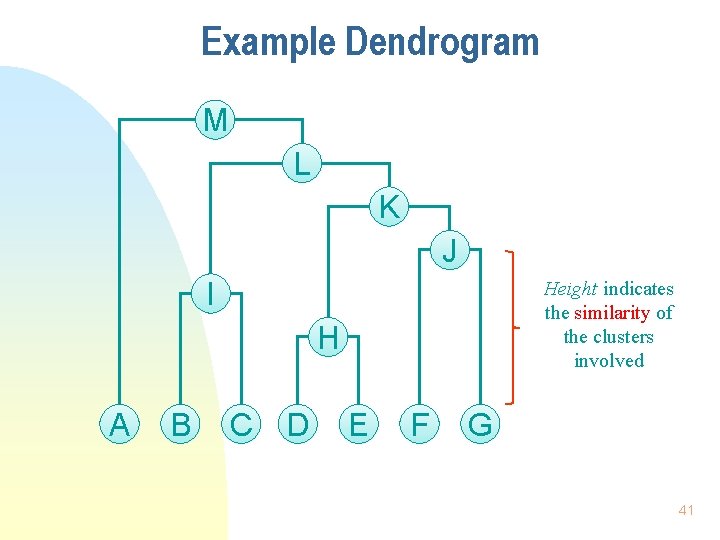
Hierarchical Clustering n Constructs a hierarchy of clusters Ø Ø Ø Starting with some initial clustering of data and iteratively trying to improve the “quality” of clusters The top level of the hierarchy consists of a single cluster with all items in it The bottom level of the hierarchy consists of N (# of items) singleton clusters n Different objectives lead to different types of clusters n Two types of hierarchical clustering n Ø Divisive (“top down”) Ø Agglomerative (“bottom up”) Hierarchy can be visualized as a dendogram 40

Example Dendrogram M L K J I Height indicates the similarity of the clusters involved H A B C D E F G 41

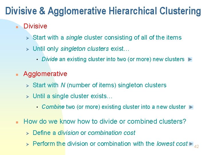
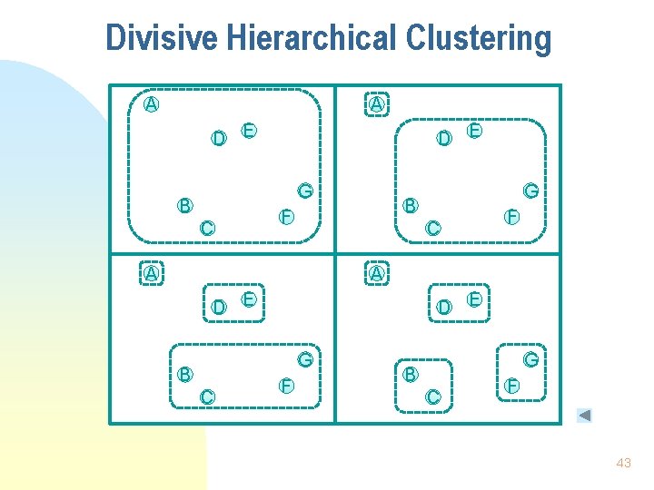
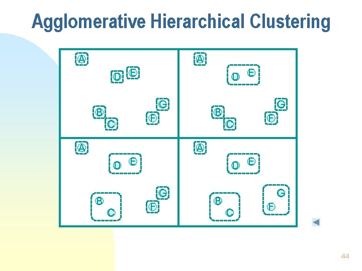
Divisive & Agglomerative Hierarchical Clustering n Divisive Ø Start with a single cluster consisting of all of the items Ø Until only singleton clusters exist… • n Agglomerative Ø Start with N (number of items) singleton clusters Ø Until a single cluster exists… • n Divide an existing cluster into two (or more) new clusters Combine two (or more) existing cluster into a new cluster How do we know how to divide or combined clusters? Ø Define a division or combination cost Ø Perform the division or combination with the lowest cost 42

Divisive Hierarchical Clustering A A D E G B C G B F C A F A D E G B C F 43

Agglomerative Hierarchical Clustering A A D E G B C G B F C A F A D E G B C F 44

Agglomerative Clustering Algorithm 45

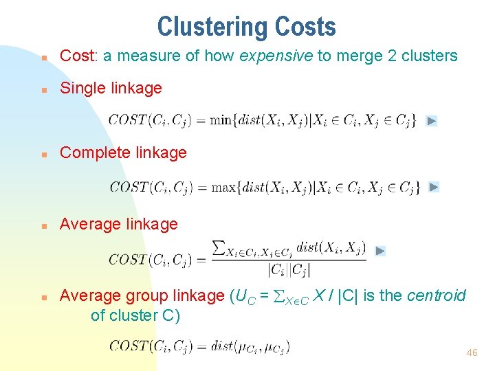
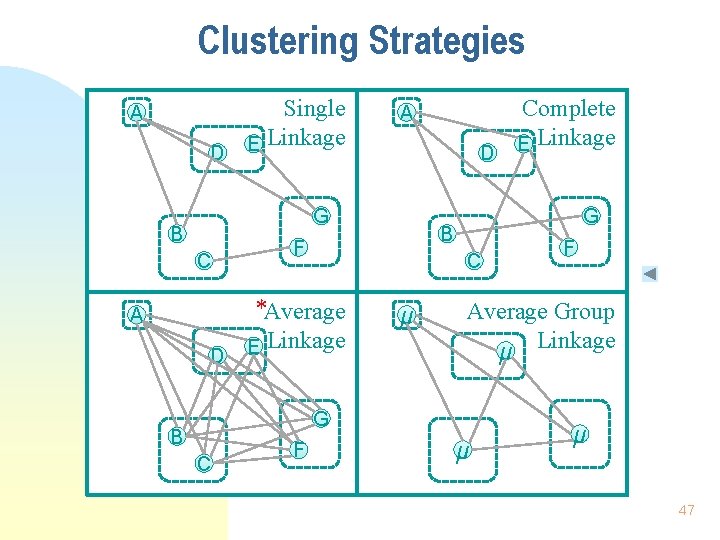
Clustering Costs n Cost: a measure of how expensive to merge 2 clusters n Single linkage n Complete linkage n Average group linkage (UC = X C X / |C| is the centroid of cluster C) 46

Clustering Strategies A D Single E Linkage A D G B C A D G B F C *Average E Linkage μ C F F Average Group μ Linkage G B Complete E Linkage μ μ 47

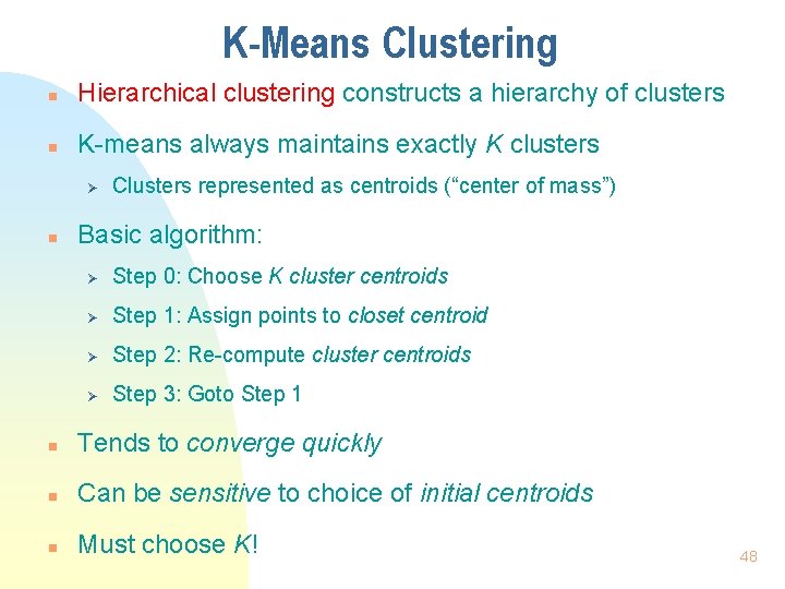
K-Means Clustering n Hierarchical clustering constructs a hierarchy of clusters n K-means always maintains exactly K clusters Ø n Clusters represented as centroids (“center of mass”) Basic algorithm: Ø Step 0: Choose K cluster centroids Ø Step 1: Assign points to closet centroid Ø Step 2: Re-compute cluster centroids Ø Step 3: Goto Step 1 n Tends to converge quickly n Can be sensitive to choice of initial centroids n Must choose K! 48

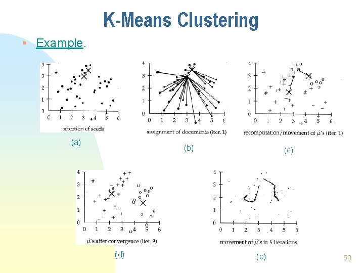
K-Means Clustering § Goal: find the cluster assignments (for the assignment vectors A[1], …, A[N]) that minimize the cost function: K COST(A[1], …, A[N]) = k=1 i: A[i]=k dist(Xi, Ck) where dist(Xi, Ck) = || Xi - Ck ||2, where Ck is the centroid of Ck = (Xi - Ck), the Euclidean Distance § Strategy: 1. Randomly select K initial cluster centers (instances) as seeds 2. Move the cluster centers around to minimize the cost function i. Re-assign instances to the cluster with the closest centroid ii. Re-compute the cost value of each centroid based on the current members of its cluster 49

K-Means Clustering § Example. (a) (b) (d) (c) (e) 50

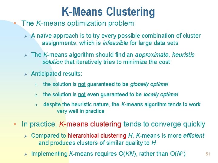
K-Means Clustering § The K-means optimization problem: Ø Ø Ø A naïve approach is to try every possible combination of cluster assignments, which is infeasible for large data sets The K-means algorithm should find an approximate, heuristic solution that iteratively tries to minimize the cost Anticipated results: 1. the solution is not guaranteed to be globally optimal 2. the solution is not even guaranteed to be locally optimal 3. despite the heuristic nature, the K-means algorithm tends to work very well in practice § In practice, K-means clustering tends to converge quickly Ø Ø Compared to hierarchical clustering H, K-means is more efficient and produces clusters of similar quality to H Implementing K-means requires O(KN), rather than O(N 2) 51

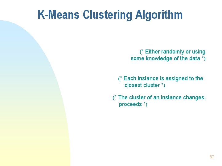
K-Means Clustering Algorithm (* Either randomly or using some knowledge of the data *) (* Each instance is assigned to the closest cluster *) (* The cluster of an instance changes; proceeds *) 52

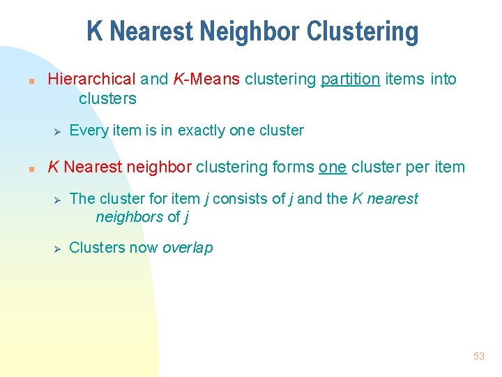
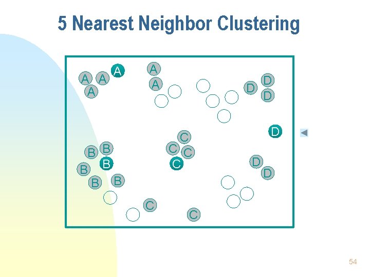
K Nearest Neighbor Clustering n Hierarchical and K-Means clustering partition items into clusters Ø n Every item is in exactly one cluster K Nearest neighbor clustering forms one cluster per item Ø Ø The cluster for item j consists of j and the K nearest neighbors of j Clusters now overlap 53

5 Nearest Neighbor Clustering A A A D D D C C B B B C D D D C 54

K Nearest Neighbor Clustering § Drawbacks of the K Nearest Neighbor Clustering method Ø Often fails to find meaningful clusters • In spare areas of the input space, the instances assigned to a cluster are father far away (e. g. , D in the 5 -NN example) • In dense areas, some related instances may be missed if K is not large enough (e. g. , B in the 5 -NN example) Ø Computational expensive (compared with K-means), since it computes distances between each pair of instances § Applications of the K Nearest Neighbor Clustering method Ø Emphasize finding a small number (rather than all) of closely related instances, i. e. , precision over recall 55

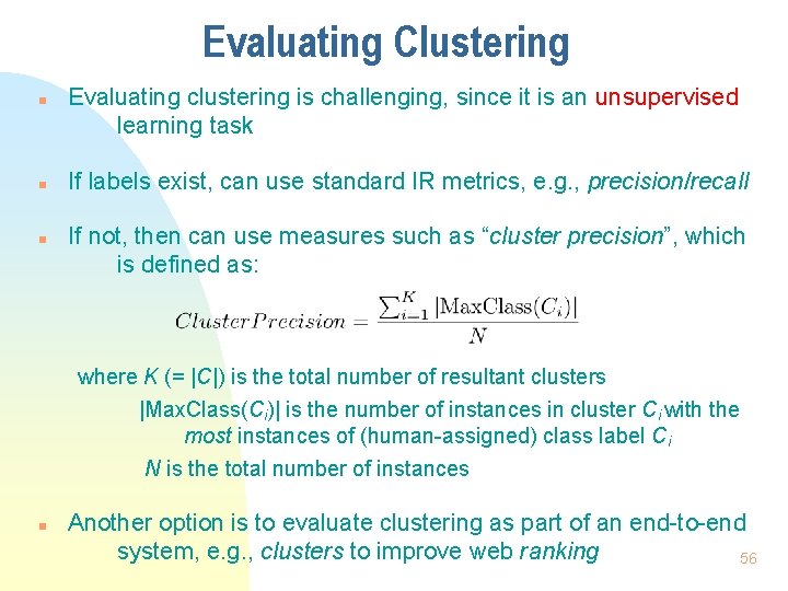
Evaluating Clustering n n n Evaluating clustering is challenging, since it is an unsupervised learning task If labels exist, can use standard IR metrics, e. g. , precision/recall If not, then can use measures such as “cluster precision”, which is defined as: where K (= |C|) is the total number of resultant clusters |Max. Class(Ci)| is the number of instances in cluster Ci with the most instances of (human-assigned) class label Ci N is the total number of instances n Another option is to evaluate clustering as part of an end-to-end system, e. g. , clusters to improve web ranking 56

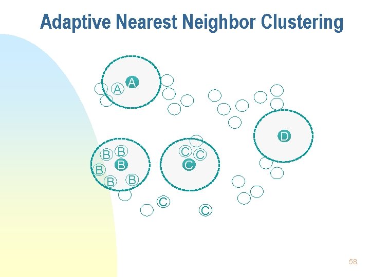
How to Choose K? § K-means and K nearest neighbor clustering require us to choose K, the number of clusters § No theoretically appealing way of choosing K § Depends on the application and data; often chosen experimentally to evaluate the quality of the resulting clusters for various values of K § Can use hierarchical clustering and choose the best level § Can use adaptive K for K-nearest neighbor clustering Ø Larger (Smaller) K for dense (spare) areas Ø Challenge: choosing the boundary size § Difficult problem with no clear solution 57

Adaptive Nearest Neighbor Clustering A A D B B B C C C 58

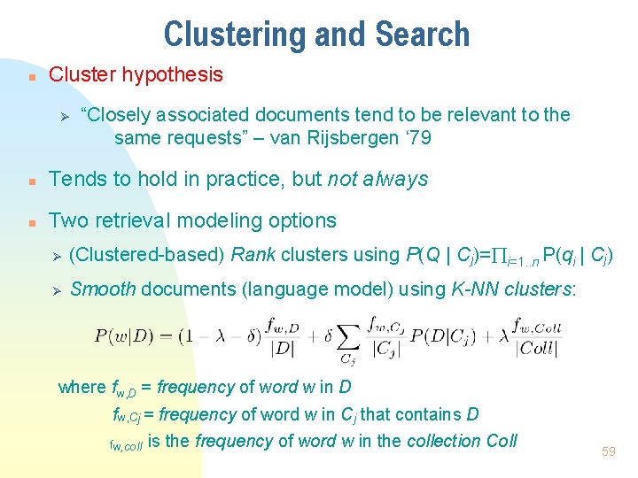
Clustering and Search n Cluster hypothesis Ø “Closely associated documents tend to be relevant to the same requests” – van Rijsbergen ‘ 79 n Tends to hold in practice, but not always n Two retrieval modeling options Ø (Clustered-based) Rank clusters using P(Q | Cj)= i=1. . n P(qi | Cj) Ø Smooth documents (language model) using K-NN clusters: where fw, D = frequency of word w in D fw, Cj = frequency of word w in Cj that contains D fw, coll is the frequency of word w in the collection Coll 59