Chapter 9 BoxJenkins ARIMA Methodology ARIMA Models The
 Methodology")
Chapter 9: Box-Jenkins (ARIMA) Methodology

ARIMA Models • The Box-Jenkins methodology refers to a set of procedures for identifying, fitting and checking ARIMA models with time series. • • The AR in ARIMA refers to Autoregressive models • The MA in ARIMA refers to Moving Average models • The I in ARIMA refers to the number of lags used in differencing the data

Autoregressive Models Yt = 0 + 1 Yt-1 + 2 Yt-2 … + p. Yt-p + et, • where t = coefficients to be estimated and p = number of lags • The number of lags (p) used in the model is a parameter and its value must be determined by the user. An autoregressive model with a lag of two will be denoted as AR(2). •

Moving Average Models • Yt = + et - w 1 et-1 - w 2 et-2 - … wqet-q, • where wt = coefficients to be estimated, and et are the error terms • The number of error terms used in the model, q, is a parameter and its value must be determined by the user. A moving average model with two error terms will be denoted as MA(2). •
 model is as")
ARMA models • Combining AR and MA models, an ARMA(p, q) model is as follows: • Yt = 0 + 1 Yt-1 + 2 Yt-2 … + p. Yt-p + et, - w 1 et-1 - w 2 et-2 - … wqet-q,

Differences • Differences of the time series may be used if it is not stationary. In some cases, a difference of the differences may be necessary before a stationary data is obtained. We use the notation “d” to indicate the number of times the time series is differenced to obtain a stationary series. • • ARIMA Notation: ARIMA(p, d, q) = An ARIMA model with the time series differenced d times as the response variable with a p-order autoregressive model mixed with q-order moving average model. •
 and PACF (Partial Autocorrelation function). PACF")
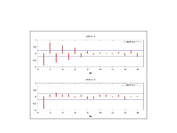
Model Identification • We use ACF (Autocorrelation function) and PACF (Partial Autocorrelation function). PACF measures the autocorrelation between Yt and Yt-k, when the effects of other time lags, 1, 2, . . , k-1, are removed
: Yt= 0+ 1 Yt-1+ t ACF PACF 1 0 k k 0 -1")
AR(1): Yt= 0+ 1 Yt-1+ t ACF PACF 1 0 k k 0 -1 -1 1 1 0 -1 21. 12. 2021 k k 0 -1 1 8
: Yt= 0+ 1 Yt-1+ 2 Yt-2 + t ACF PACF 1 0 k")
AR(2): Yt= 0+ 1 Yt-1+ 2 Yt-2 + t ACF PACF 1 0 k k 0 -1 -1 1 1 0 -1 21. 12. 2021 k k 0 -1 1 9
: Yt= + t- 1 t-1 ACF PACF 1 k 0 -1 1 k")
MA(1): Yt= + t- 1 t-1 ACF PACF 1 k 0 -1 1 k 0 -1 21. 12. 2021 k 1 -1 0 0 1 -1 k 10
: Yt= + t- 1 t-1 - 2 t-2 ACF 1 k 0 -1")
MA(2): Yt= + t- 1 t-1 - 2 t-2 ACF 1 k 0 -1 k 1 k 0 k -1 Pazarlıoğlu-Güneş 0 21. 12. 2021 0 -1 1 -1 1 PACF 11
: Yt= 0+ 1 Yt-1 + t- 1 t-1 Otokorelasyon Kısmi Otokorelasyon 1")
ARMA(1, 1): Yt= 0+ 1 Yt-1 + t- 1 t-1 Otokorelasyon Kısmi Otokorelasyon 1 0 -1 21. 12. 2021 k 0 k -1 Pazarlıoğlu-Güneş 1 12
: Yt= 0+ 1 Yt-1 + t- 1 t-1 Auto Correlation Partial Auto")
ARMA(1, 1): Yt= 0+ 1 Yt-1 + t- 1 t-1 Auto Correlation Partial Auto Correlation 1 k 0 21. 12. 2021 -1 -1 k 0 1 13
 AR(p) Cut off after the order of q")
AR, MA or ARMA? Autocorrelations MA(q) AR(p) Cut off after the order of q of the process Die out ARMA(p, q) Die out Partial Autocorrelations Die out Cut off after the order of p of the process Die out

Model Building Strategy • Step 1: Model identification Plot the time series/ACF and examine whether it is stationary. If not, try some transformation and or differencing, until the data seems stationary. Compare ACF and PACF of the time series data and identify the ARIMA model to be used. To judge the significance of autocorrelation and partial autocorrelation, the corresponding sample values may be compared with ± 2/. Use the principle of parsimony. • Step 2: Model estimation Use SPSS or other package to estimate the model parameters. t-test may be used to judge whether a parameter may be dropped from the model.

Model Building Strategy • Step 3: Model checking • The model will be considered adequate if the residuals are random. The following three procedures may be used. • Residual plots as in regression may be used, • rk(e) must be within ± 2/ of zero, and • L-Q test may be used to test whether a group autocorrelation of lags 1, 2, . . m, is significant. • • Step 4: Model forecasting • SPSS generates forecasts for a given number of future periods.
 selects the best model from a")
Model Selection Criteria • Akaike Information Criterion (AIC) selects the best model from a group of candidate models as the one that minimizes • Bayesian Information Criterion (BIC) selects the best model e that minimizes where σ2 residual variance

ATR şirketi üretim hedefleri Öngörüsü -0. 23 0. 63 0. 48 -0. 83 -0. 03 1. 31 0. 86 -1. 28 0 -0. 63 0. 08 -1. 3 1. 48 -0. 28 -0. 79 1. 86 0. 07 0. 09 21. 12. 2021 -0. 21 0. 91 -0. 36 0. 48 0. 61 -1. 38 -0. 04 0. 9 1. 79 -0. 37 0. 4 -1. 19 0. 98 -1. 51 0. 9 -1. 56 2. 18 -1. 93 1. 87 -0. 97 0. 46 2. 12 -2. 11 0. 7 0. 69 -0. 24 0. 34 0. 6 0. 15 -0. 02 0. 46 -0. 54 0. 89 1. 07 0. 2 -0. 97 0. 83 -0. 33 0. 91 -1. 13 2. 22 0. 8 -1. 95 2. 61 0. 59 0. 71 -0. 84 -0. 11 1. 27 -0. 8 -0. 76 1. 58 -0. 38 0. 1 -0. 62 2. 27 -0. 62 0. 74 -0. 16 1. 34 -1. 83 0. 31 1. 13 -0. 87 1. 45 -1. 95 -0. 51 -0. 41 0. 49 1. 54 -0. 96 20

ATR şirketi üretim hedefleri Öngörüsü Tanımlama Süreci verilerin dağılma grafiği, otokorelasyon ve kısmi otokorelasyon fonksiyonlarını incelemekle başlar. 21. 12. 2021 21

ATR şirketi üretim hedefleri Öngörüsü Sapma 3 2 1 0 -1 -2 -3 21. 12. 2021 1 9 17 25 33 41 49 57 65 73 81 89 22

ATR şirketi üretim hedefleri Öngörüsü Hem zaman serisi grafiğine hem de otokorelasyon fonksiyonları serinin durağan olduğunu göstermektedir. Sadece 1. gecikmedeki -0. 50 otokorelasyon katsayısı anlamlıdır. Diğer gecikmelerdeki otokorelasyon katsayılarının her biri küçük olup hata sınırları içersindedir. Örnek otokorelasyon katsayıları birinci gecikmeden sonra kesilmektedir. İlk üç Örnek kısmi otokorelasyon katsayılarının hepsi negatif olup sıfıra doğru azalmaktadır. 21. 12. 2021 23

ATR şirketi üretim hedefleri Öngörüsü Örnek otokorelasyon katsayıları ile Örnek kısmi otokorelasyon katsayılarının davranışı MA(1) teorik davranışa benzemektedir. Otokorelasyon Kısmi Otokorelasyon 1 k -1 21. 12. 2021 -1 0 k 0 1 24
: Yt= + t+ 1 t-1 21. 12. 2021")
ATR şirketi üretim hedefleri Öngörüsü MA(1): Yt= + t+ 1 t-1 21. 12. 2021 25

ATR şirketi üretim hedefleri Öngörüsü ARIMA Model: sapma Estimates at each iteration Iteration SSE Parameters 0 96. 3554 0. 100 0. 247 1 85. 3276 0. 250 0. 201 2 78. 1410 0. 400 0. 171 3 74. 6680 0. 550 0. 153 4 74. 5019 0. 591 0. 151 5 74. 5004 0. 587 0. 151 6 74. 5004 0. 588 0. 151 21. 12. 2021 26

ATR şirketi üretim hedefleri Öngörüsü Relative change in each estimate less than 0. 0010 Final Estimates of Parameters Type Coef SE Coef T P MA 1 0. 5875 0. 0864 6. 80 0. 000 Constant 0. 15129 0. 04022 3. 76 0. 000 Mean 0. 15129 0. 04022 Number of observations: 90 Residuals: SS = 74. 4933 (backforecasts excluded) MS = 0. 8465 DF = 88 Modified Box-Pierce (Ljung-Box) Chi-Square statistic Lag 12 24 36 48 Chi-Square 9. 1 10. 8 17. 3 31. 5 DF 10 22 34 46 P-Value 0. 524 0. 977 0. 992 0. 950 Forecasts from period 90 95% Limits Period Forecast Lower Upper Actual 91 0. 43350 -1. 37018 2. 23719 92 0. 15129 -1. 94064 2. 24322 21. 12. 2021 27

ATR şirketi üretim hedefleri Öngörüsü 21. 12. 2021 28

ATR şirketi üretim hedefleri Öngörüsü Gözlem no 1 2 3 4 5. . . 86 87 88 89 90 91öngörü 92öngörü 21. 12. 2021 Sapma -0. 23 0. 63 0. 48 -0. 83 -0. 03. . . -0. 51 -0. 41 0. 49 1. 54 -0. 96 0. 4335 0. 1513 tahmin 0. 101969 0. 346323 -0. 015371 -0. 139741 0. 556819. . . 1. 06829 1. 07854 1. 02581 0. 46608 -0. 47964 0. 4335 hata -0. 331969 0. 283677 0. 495371 -0. 690259 -0. 586819. . . -1. 57829 -1. 48854 -0. 53581 1. 07392 -0. 48036 0. 0000 29

ISC şirketi hisse senetleri kapanış fiyatları 235 320 115 355 190 320 275 205 295 240 355 175 285 21. 12. 2021 200 290 220 400 275 185 370 255 285 250 300 225 285 250 225 125 295 250 355 280 370 250 290 225 270 180 270 240 275 225 285 250 310 220 320 215 260 190 295 275 205 265 245 170 175 270 225 340 190 250 300 195 30

ISC şirketi hisse senetleri kapanış fiyatları ISC 500 400 300 200 100 0 21. 12. 2021 1 9 17 25 33 41 49 57 65 31

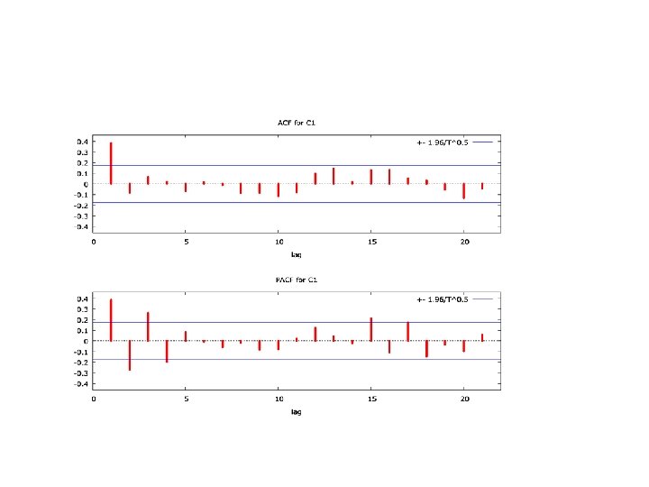
ISC şirketi hisse senetleri kapanış fiyatları Hisse seneti fiyatlarının hem zaman serisi grafiğine hem de otokorelasyon fonksiyonları serinin durağan olduğunu göstermektedir. Zaman serisi grafiği yaklaşık 250 birim lira civarında değişmektedir. Autocorrelation Function: ISC Lag ACF T LBQ 1 -0. 401525 -3. 24 2 0. 333244 2. 34 3 -0. 204772 -1. 33 4 0. 111059 0. 70 5 -0. 182873 -1. 15 10. 97 18. 65 21. 59 22. 47 24. 90 1. gecikmedeki -0. 40 otokorelasyon katsayısı ile 2. gecikmedeki 0. 33 otokorelasyon katsayısı anlamlıdır. Örnek otokorelasyon katsayıları ikinci gecikmeden sonra kesilmektedir. Diğer gecikmelerdeki otokorelasyon katsayılarının her biri küçük olup hata sınırları içersindedir. 21. 12. 2021 32

ISC şirketi hisse senetleri kapanış fiyatları Lag PACF 1 -0. 401525 2 0. 205086 3 -0. 019988 4 -0. 034493 5 -0. 136220 T -3. 24 1. 65 -0. 16 -0. 28 -1. 10 İlk örnek kısmi otokorelasyon katsayısı negatif olup sıfıra doğru azalmaktadır. 21. 12. 2021 33

ISC şirketi hisse senetleri kapanış fiyatları Örnek otokorelasyon katsayıları ile Örnek kısmi otokorelasyon katsayılarının davranışı AR(2) teorik davranışa benzemektedir. 1 1 0 -1 21. 12. 2021 k -1 Pazarlıoğlu-Güneş k 0 34
: Yt= 0+ 1 Yt-1+ 2 Yt-2 +")
ISC şirketi hisse senetleri kapanış fiyatları AR(2): Yt= 0+ 1 Yt-1+ 2 Yt-2 + t 35

ISC şirketi hisse senetleri kapanış fiyatları Örnek otokorelasyon katsayıları ile Örnek kısmi otokorelasyon katsayılarının davranışı AR(2) teorik davranışa benzemektedir. ARIMA Model: ISC Estimates at each iteration Iteration SSE Parameters 0 224504 0. 100 205. 988 1 195673 -0. 050 0. 138 234. 824 2 178964 -0. 200 0. 178 263. 252 3 174473 -0. 318 0. 213 284. 721 4 174451 -0. 324 0. 219 284. 977 5 174451 -0. 324 0. 219 284. 914 6 174451 -0. 324 0. 219 284. 903 21. 12. 2021 36

ISC şirketi hisse senetleri kapanış fiyatları Final Estimates of Parameters Type Coef SE Coef T P AR 1 -0. 3243 0. 1246 -2. 60 0. 012 AR 2 0. 2192 0. 1251 1. 75 0. 085 Constant 284. 903 6. 573 43. 34 0. 000 Mean 257. 828 5. 949 Number of observations: 65 Residuals: SS = 174093 (backforecasts excluded) MS = 2808 DF = 62 Modified Box-Pierce (Ljung-Box) Chi-Square statistic Lag 12 24 36 48 Chi-Square 6. 3 13. 3 18. 2 29. 1 DF 9 21 33 45 P-Value 0. 707 0. 899 0. 983 0. 969 Forecasts from period 65 95% Limits Period Forecast Lower Upper Actual 66 287. 446 183. 565 391. 328 67 234. 450 125. 244 343. 656 68 271. 902 157. 615 386. 189 21. 12. 2021 37

ISC şirketi hisse senetleri kapanış fiyatları 38

ISC şirketi hisse senetleri kapanış fiyatları Gözlem no 1 2 3 4 5. . . 61 62 63 64 65 66öngörü 67öngörü ISC 235 320 115 355 190. . . 340 190 250 300 195 287. 4 234. 5 tahmin hata 248. 416 -13. 416 269. 842 50. 158 232. 664 -117. 664 317. 771 37. 229 195. 006 -5. 006. . . 271. 141 68. 8586 223. 987 -33. 9866 297. 837 -47. 8371 245. 496 54. 5041 242. 438 -47. 4377 287. 445 -0. 0450 39
- Slides: 39