CHAPTER 8 THE DISCOVERY OF PRODUCTION AND ITS

CHAPTER 8 THE DISCOVERY OF PRODUCTION AND ITS TECHNOLOGY

DISCOVERING PRODUCTION • Primitive society • Fruit and land • Accidental discovery: jam • Opportunity cost • Cost of engaging in any activity • Opportunity forgone - particular activity • Normal profit • Just sufficient to recover opportunity cost • Extra-normal profit • Return above normal profit 2

PRODUCTION FUNCTION AND TECHNOLOGY • Technology • Set of technological constraints • On production • Combine inputs into outputs 3

PRODUCTION FUNCTION AND TECHNOLOGY • No free lunch assumption • Production process • Need inputs to produce outputs • Non reversibility assumption • Cannot run a production process in reverse • Free disposability assumption • Combination of inputs • Certain output • Or strictly less output 4

PRODUCTION FUNCTION AND TECHNOLOGY • Additivity assumption • Produce output x • One combination of inputs • Produce output y • Another combination of inputs • Feasible: produce x+y 5

PRODUCTION FUNCTION AND TECHNOLOGY • Divisibility assumption • Feasible input combination y • Then, λy – feasible input combination • 0≤ λ ≤ 1 6

PRODUCTION FUNCTION AND TECHNOLOGY • Convexity assumption • Production activity: y • Output: z • Particular amounts of inputs • Production activity: w • Output: z • Different amounts of inputs • Produce: at least z • Mix activities y (λ time) and w(1 - λ time) 7

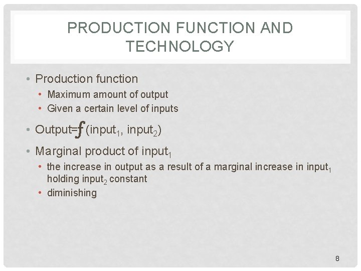
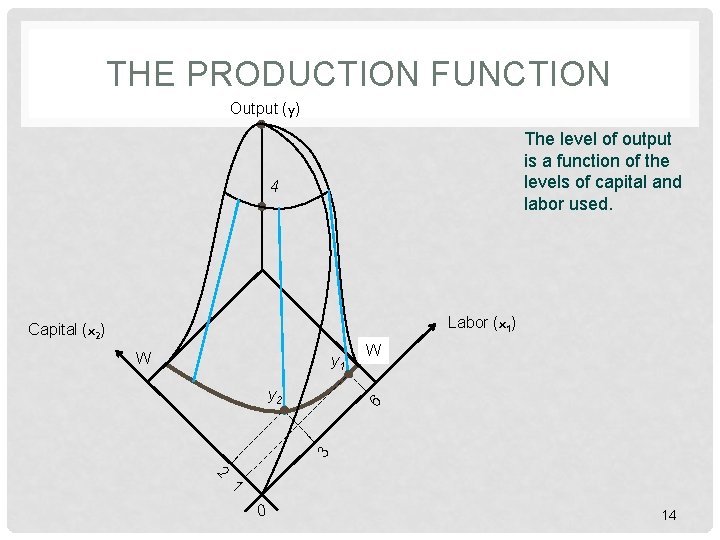
PRODUCTION FUNCTION AND TECHNOLOGY • Production function • Maximum amount of output • Given a certain level of inputs • Output=f (input 1, input 2) • Marginal product of input 1 • the increase in output as a result of a marginal increase in input 1 holding input 2 constant • diminishing 8

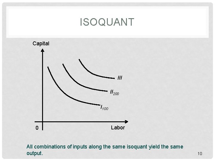
ISOQUANT • Isoquant • Set of bundles • Given production function • Produce same output • Most efficiently

ISOQUANT Capital III II 200 I 100 0 Labor All combinations of inputs along the same isoquant yield the same output. 10

ISOQUANT • Isoquants • Never cross each other • Farther from the origin greater outputs • Slope • Marginal rate of technical substitution 11

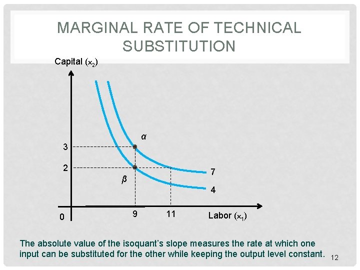
MARGINAL RATE OF TECHNICAL SUBSTITUTION Capital (x 2) α 3 2 7 β 4 0 9 11 Labor (x 1) The absolute value of the isoquant’s slope measures the rate at which one input can be substituted for the other while keeping the output level constant. 12

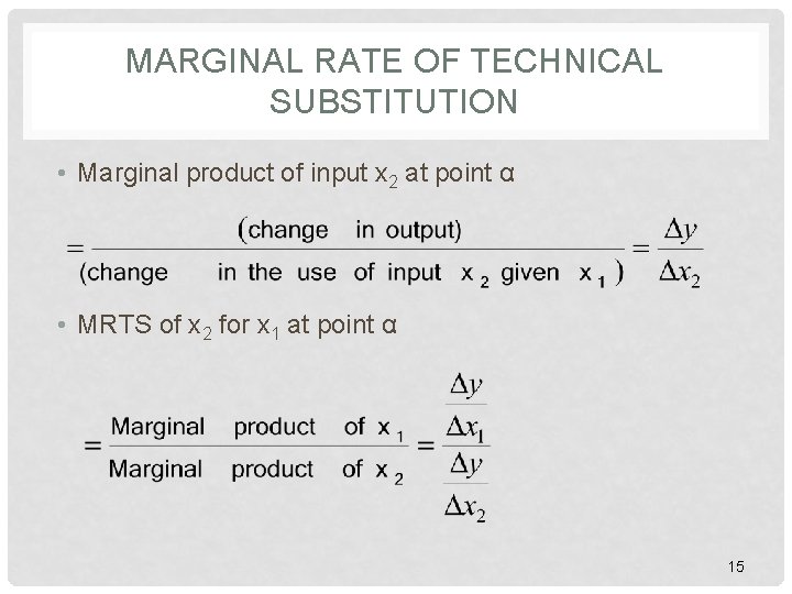
MARGINAL RATE OF TECHNICAL SUBSTITUTION • Marginal rate of technical substitution (MRTS) • Rate of substitution • One input for another • Constant output 13

THE PRODUCTION FUNCTION Output (y) The level of output is a function of the levels of capital and labor used. 4 Labor (x 1) Capital (x 2) W y 1 y 2 2 W 6 3 1 0 14

MARGINAL RATE OF TECHNICAL SUBSTITUTION • Marginal product of input x 2 at point α • MRTS of x 2 for x 1 at point α 15

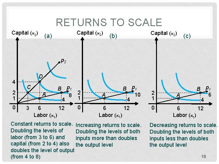
DESCRIBING TECHNOLOGIES • Returns to scale – ratio of • Change in output • Proportionate change in all inputs • Constant returns to scale • All inputs - increase by λ • Output - increases by λ 16

DESCRIBING TECHNOLOGIES • Increasing returns to scale • All inputs - increase by λ • Output - increases by more than λ • Decreasing returns to scale • All inputs - increase by λ • Output - increases by less than λ • Elasticity of substitution • Substitute one input for another • Given level of output 17

RETURNS TO SCALE Capital (x 2) (a) Capital (x 2) (b) (c) p 2 4 2 1 0 D C A 3 B p 1 8 4 6 12 Labor (x 1) 2 1 0 A B p 1 10 4 12 6 Labor (x 1) Constant returns to scale. Increasing returns to scale. Doubling the levels of both labor (from 3 to 6) and inputs more than doubles capital (from 2 to 4) also the output level doubles the level of output (from 4 to 8) 2 1 0 A B p 1 6 4 6 12 Labor (x 1) Decreasing returns to scale. Doubling the levels of both inputs less than doubles the output level 18

TIME CONSTRAINTS • Immediate run • Period of time • Cannot vary inputs • Fixed factor of production • Cannot be adjusted • Given period of time • Variable factor of production • Can be adjusted 19

TIME CONSTRAINTS • Short run • Time period • At least one factor of production – fixed • Long run • Time period • All factors of production – variable 20

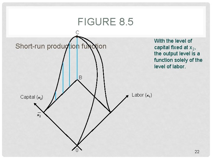
TIME CONSTRAINTS • Long-run production function • All inputs – variable • Short-run production function • Some inputs – variable • Capital – fixed • Labor – variable 21

FIGURE 8. 5 C With the level of capital fixed at x 2, the output level is a function solely of the level of labor. Short-run production function B Labor (x 1) Capital (x 2) x 2 0 22

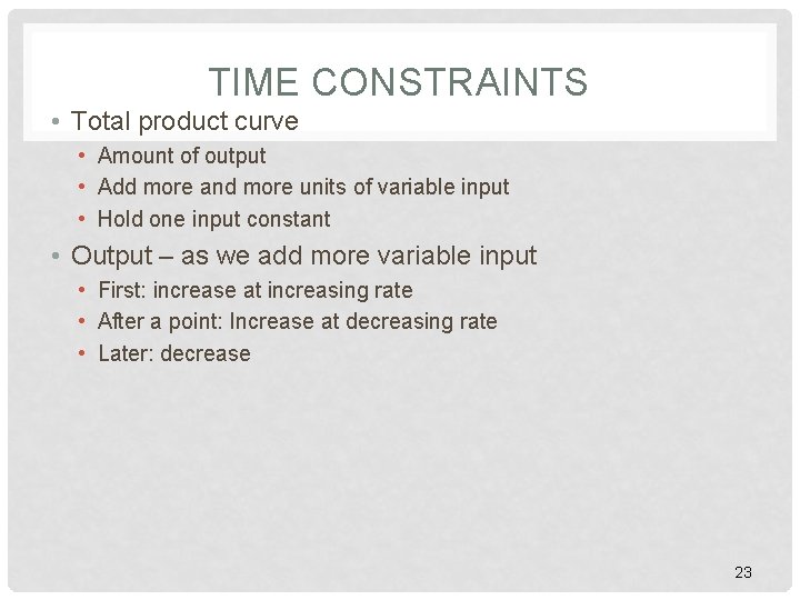
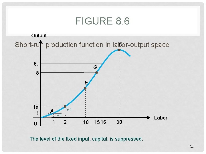
TIME CONSTRAINTS • Total product curve • Amount of output • Add more and more units of variable input • Hold one input constant • Output – as we add more variable input • First: increase at increasing rate • After a point: Increase at decreasing rate • Later: decrease 23

FIGURE 8. 6 Output D Short-run production function in labor-output space 8 14 G 8 E 1 12 1 2 0 A 1 +1 +1 2 10 15 16 30 Labor The level of the fixed input, capital, is suppressed. 24

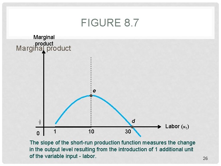
TIME CONSTRAINTS • Decreasing returns to factor • Rate of output growth: decreasing • Increase one input • Other inputs – constant • Marginal product curve • Marginal product • Factor of production 25

FIGURE 8. 7 Marginal product e d 1 2 0 1 10 30 Labor (x 1) The slope of the short-run production function measures the change in the output level resulting from the introduction of 1 additional unit of the variable input - labor. 26

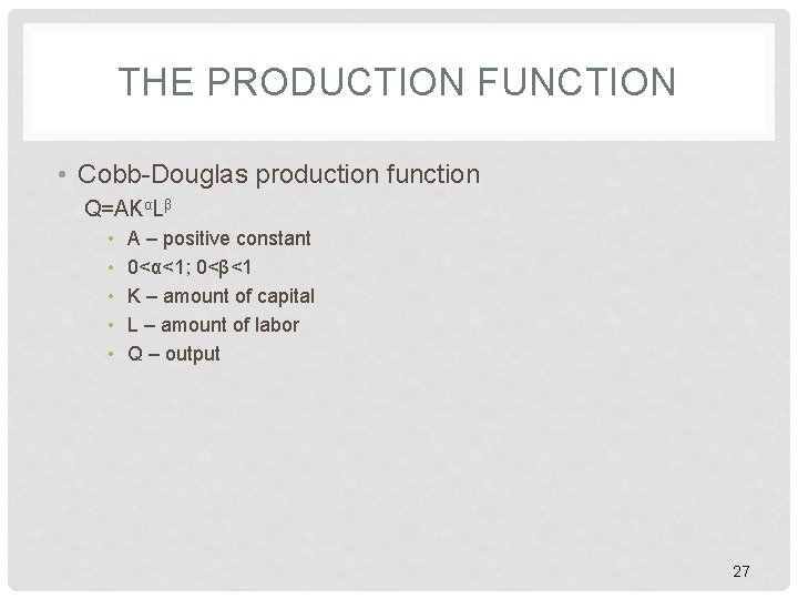
THE PRODUCTION FUNCTION • Cobb-Douglas production function Q=AKαLβ • • • A – positive constant 0<α<1; 0<β<1 K – amount of capital L – amount of labor Q – output 27

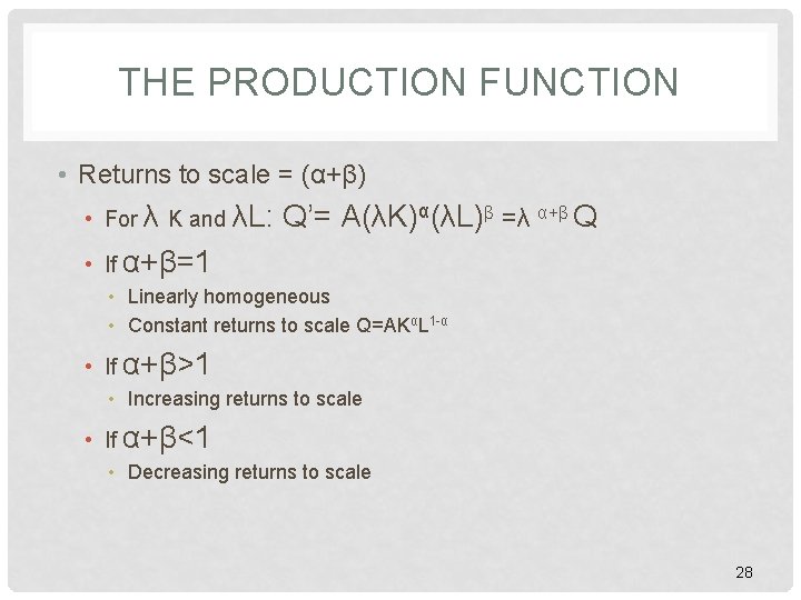
THE PRODUCTION FUNCTION • Returns to scale = (α+β) • For λ K and λL: Q’= A(λK)α(λL)β =λ α+β Q • If α+β=1 • Linearly homogeneous • Constant returns to scale Q=AKαL 1 -α • If α+β>1 • Increasing returns to scale • If α+β<1 • Decreasing returns to scale 28

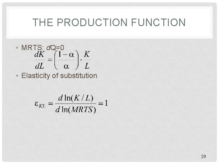
THE PRODUCTION FUNCTION • MRTS: d. Q=0 • Elasticity of substitution 29

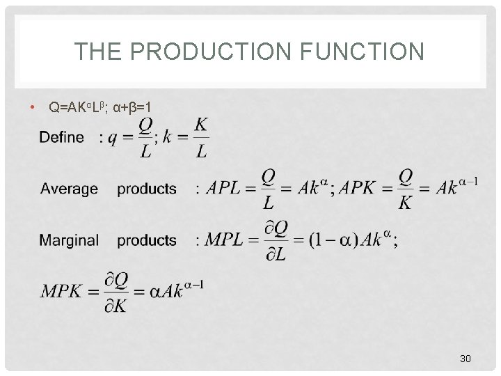
THE PRODUCTION FUNCTION • Q=AKαLβ; α+β=1 30

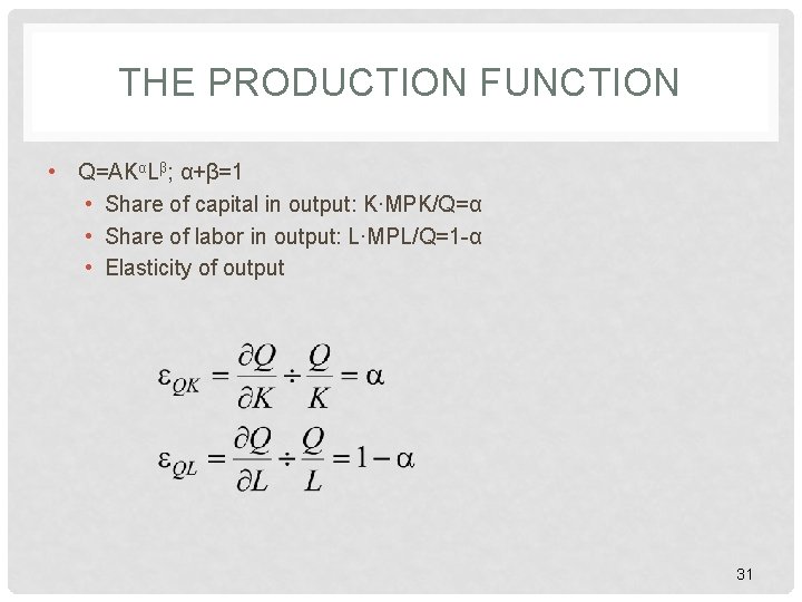
THE PRODUCTION FUNCTION • Q=AKαLβ; α+β=1 • Share of capital in output: K∙MPK/Q=α • Share of labor in output: L∙MPL/Q=1 -α • Elasticity of output 31