Chapter 8 Storage Indexing Data on External Storage

Chapter 8 Storage & Indexing

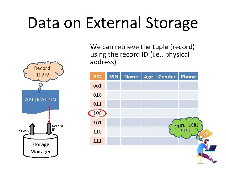
Data on External Storage We can retrieve the tuple (record) using the record ID (i. e. , physical address) Record ID ? ? ? RID SSN Name Age Gender Phone 001 APPLICATION 010 011 100 Record ID Record Storage Manager 101 110 111 1101 1001 0101

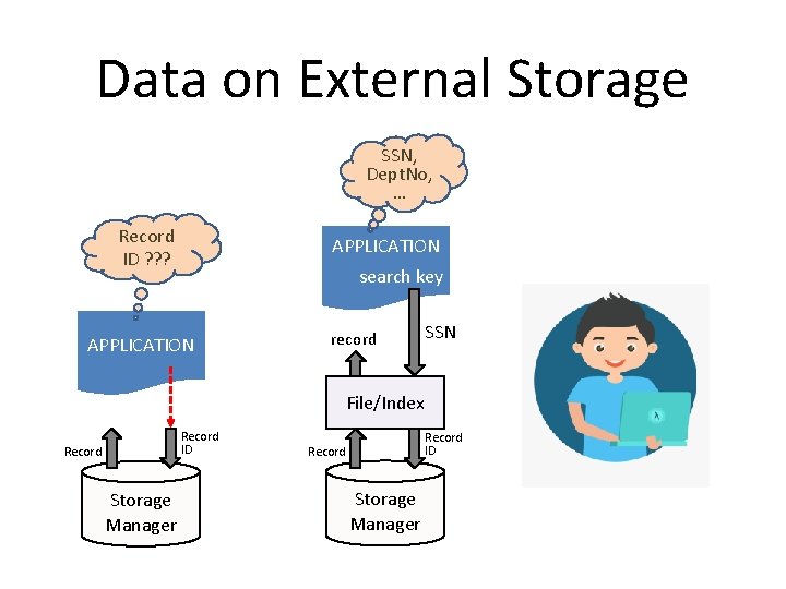
Data on External Storage SSN, Dept. No, … Record ID ? ? ? APPLICATION search key APPLICATION record SSN File/Index Record ID Record Storage Manager

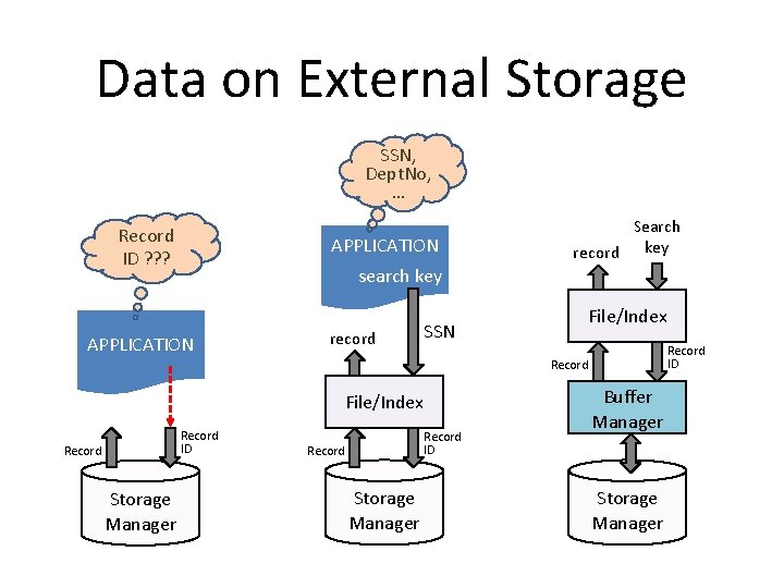
Data on External Storage SSN, Dept. No, … Record ID ? ? ? APPLICATION Search record key search key APPLICATION record File/Index SSN Record ID Record File/Index Record ID Record Storage Manager Buffer Manager Storage Manager

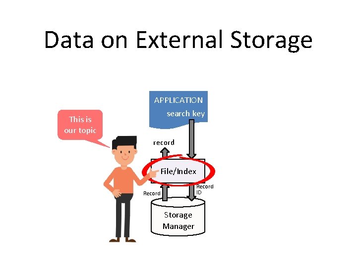
Data on External Storage APPLICATION This is our topic search key record File/Index Record ID Record Storage Manager

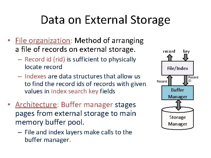
Data on External Storage • File organization: Method of arranging a file of records on external storage. – Record id (rid) is sufficient to physically locate record – Indexes are data structures that allow us to find the record ids of records with given values in index search key fields • Architecture: Buffer manager stages pages from external storage to main memory buffer pool. – File and index layers make calls to the buffer manager. record key File/Index Record ID Record Buffer Manager Storage Manager

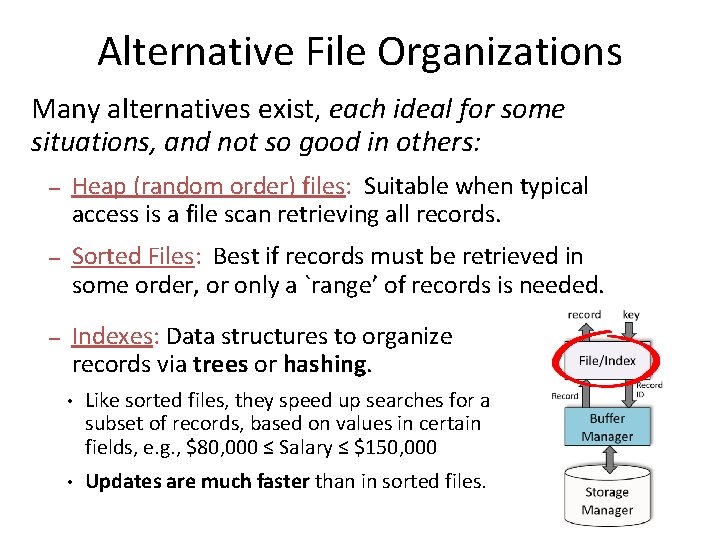
Alternative File Organizations Many alternatives exist, each ideal for some situations, and not so good in others: – Heap (random order) files: Suitable when typical access is a file scan retrieving all records. – Sorted Files: Best if records must be retrieved in some order, or only a `range’ of records is needed. – Indexes: Data structures to organize records via trees or hashing. • Like sorted files, they speed up searches for a subset of records, based on values in certain fields, e. g. , $80, 000 ≤ Salary ≤ $150, 000 • Updates are much faster than in sorted files.

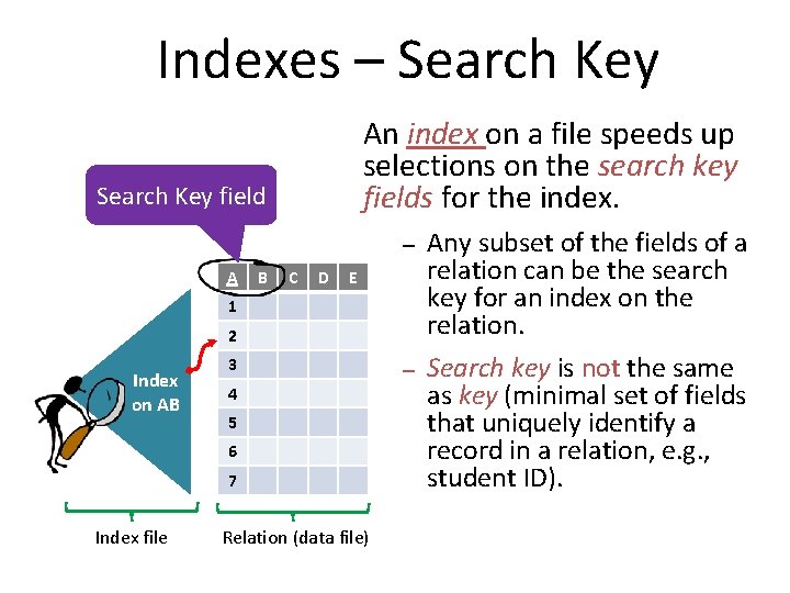
Indexes – Search Key An index on a file speeds up selections on the search key fields for the index. Search Key field A B C D – Any subset of the fields of a relation can be the search key for an index on the relation. – Search key is not the same as key (minimal set of fields that uniquely identify a record in a relation, e. g. , student ID). E 1 2 Index on AB 3 4 5 6 7 Index file Relation (data file)

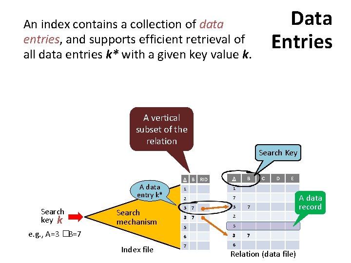
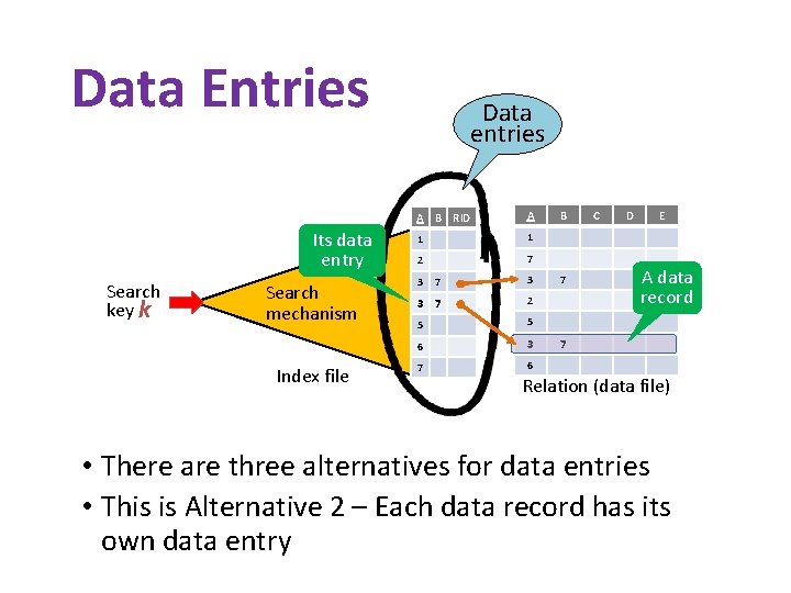
Data Entries An index contains a collection of data entries, and supports efficient retrieval of all data entries k* with a given key value k. A vertical subset of the relation Search Key A data entry k* Search key k Search mechanism e. g. , A=3 � B=7 Index file A B RID A 1 1 2 7 7 3 3 7 2 5 5 6 3 7 6 3 B C D E 7 7 Relation (data file) A data record

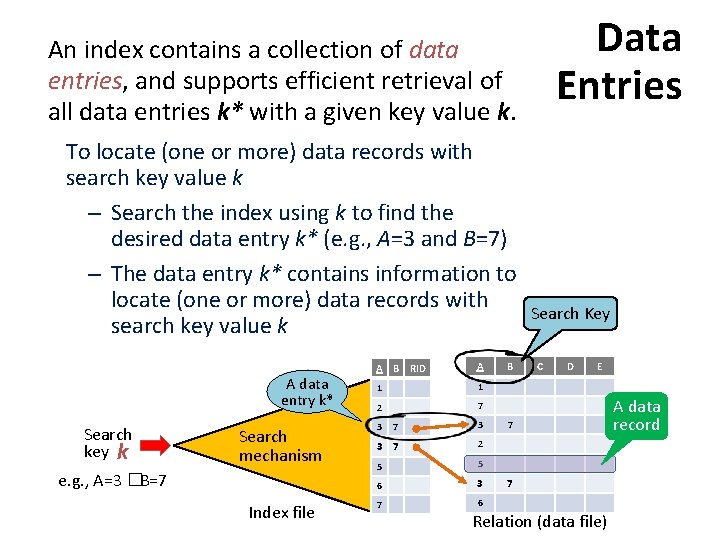
Data Entries An index contains a collection of data entries, and supports efficient retrieval of all data entries k* with a given key value k. To locate (one or more) data records with search key value k – Search the index using k to find the desired data entry k* (e. g. , A=3 and B=7) – The data entry k* contains information to locate (one or more) data records with search key value k A data entry k* Search key k Search mechanism e. g. , A=3 � B=7 Index file A B RID A 1 1 2 7 7 3 3 7 2 5 5 6 3 7 6 3 B Search Key C D E 7 7 Relation (data file) A data record

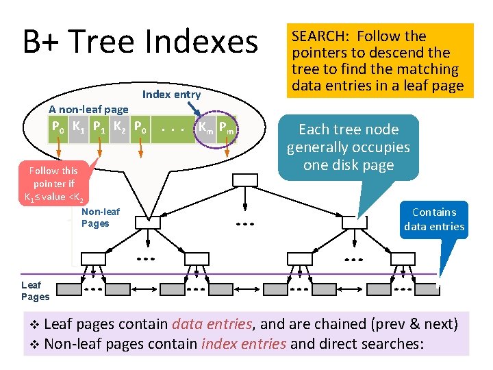
B+ Tree Indexes A non-leaf page Index entry P 0 K 1 P 1 K 2 P 0 Follow this pointer if K 1≤ value <K 2 Non-leaf Pages . . . K m Pm SEARCH: Follow the pointers to descend the tree to find the matching data entries in a leaf page Each tree node generally occupies one disk page Contains data entries Leaf Pages Leaf pages contain data entries, and are chained (prev & next) v Non-leaf pages contain index entries and direct searches: v

B+ Tree Indexes Index contains auxiliary information that directs searches to the desired data entries SEARCH: Follow the pointers to descend the tree to find the matching data entries in a leaf page Search Key Non-leaf Pages Leaf Pages Record ID

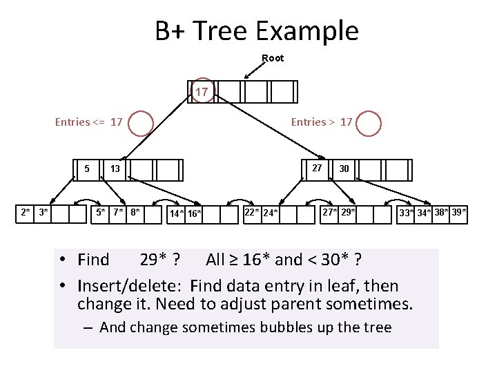
B+ Tree Example Root 17 Entries <= 17 5 2* 3* Entries > 17 27 13 5* 7* 8* 14* 16* 22* 24* 30 27* 29* 33* 34* 38* 39* • Find 29* ? All ≥ 16* and < 30* ? • Insert/delete: Find data entry in leaf, then change it. Need to adjust parent sometimes. – And change sometimes bubbles up the tree

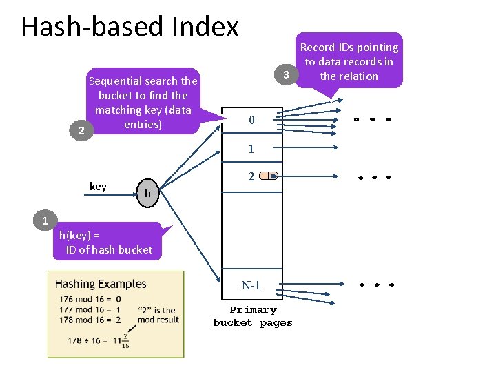
Hash-based Index 2 Sequential search the bucket to find the matching key (data entries) Record IDs pointing to data records in 3 the relation 0 1 key 1 2 h h(key) = ID of hash bucket e. g. , h(key) = key mod N The mod function computes the remainder of the division “key ÷N” N-1 Primary bucket pages Overflow page

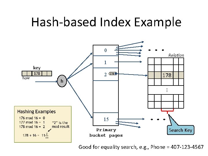
Hash-based Index Example 0 1 key Tuple 178 2 Relation Overflow page 178 h 178. . . 15 Primary bucket pages Search Key Good for equality search, e. g. , Phone = 407 -123 -4567

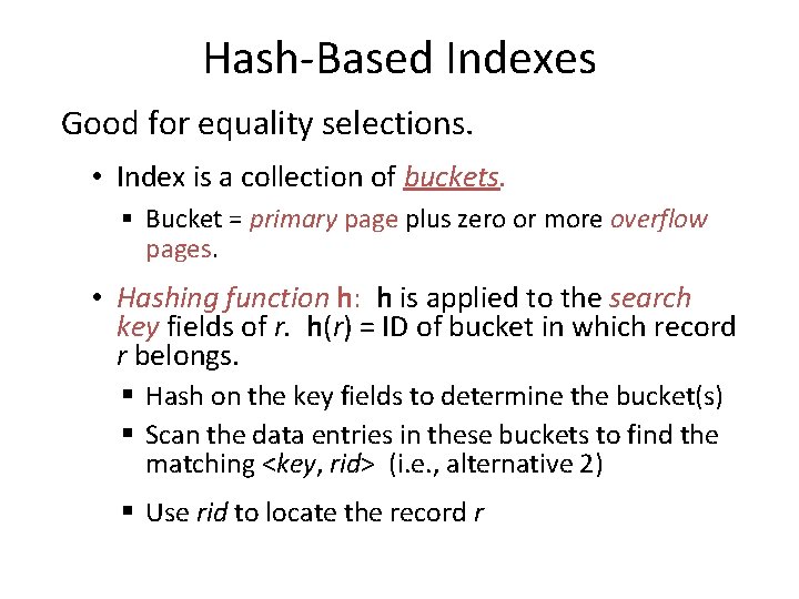
Hash-Based Indexes Good for equality selections. • Index is a collection of buckets. § Bucket = primary page plus zero or more overflow pages. • Hashing function h: h is applied to the search key fields of r. h(r) = ID of bucket in which record r belongs. § Hash on the key fields to determine the bucket(s) § Scan the data entries in these buckets to find the matching <key, rid> (i. e. , alternative 2) § Use rid to locate the record r

Data Entries Its data entry Search key k Search mechanism Index file Data entries A B RID A 1 1 2 7 7 3 3 7 2 5 5 6 3 7 6 3 B 7 C D E A data record 7 Relation (data file) • There are three alternatives for data entries • This is Alternative 2 – Each data record has its own data entry

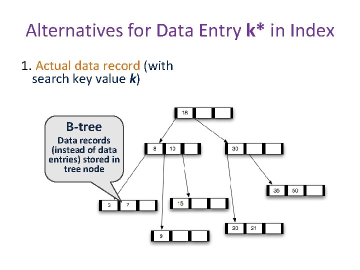
Alternatives for Data Entry k* in Index 1. Actual data record (with search key value k) B-tree Data records (instead of data entries) stored in tree node

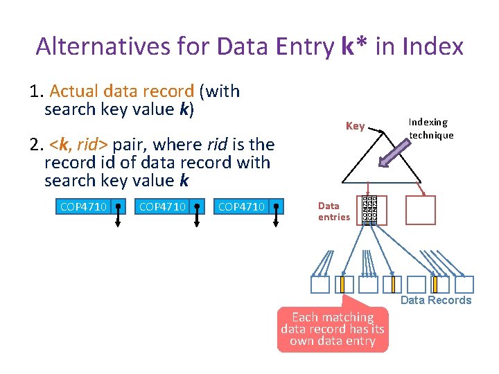
Alternatives for Data Entry k* in Index 2. <k, rid> pair, where rid is the record id of data record with search key value k COP 4710 Key Data entries Indexing technique COP 4710 1. Actual data record (with search key value k) Data Records Each matching data record has its own data entry

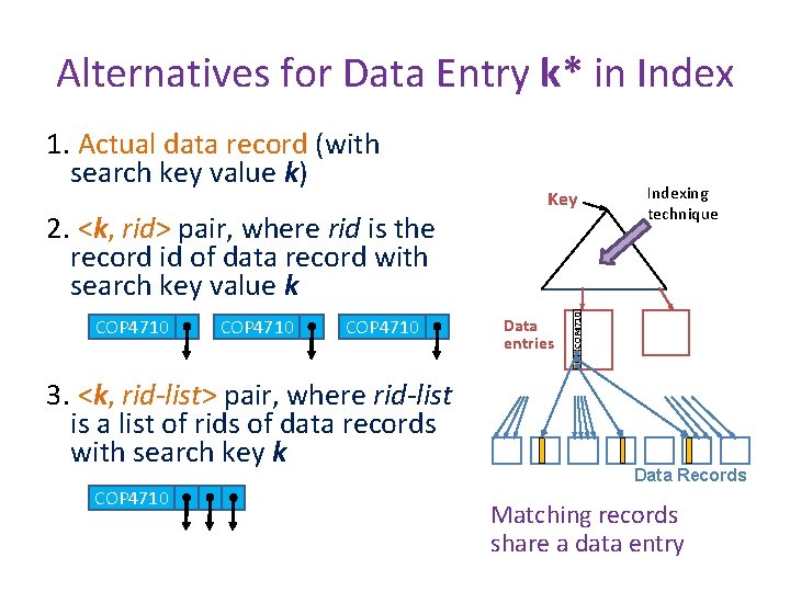
Alternatives for Data Entry k* in Index 2. <k, rid> pair, where rid is the record id of data record with search key value k COP 4710 3. <k, rid-list> pair, where rid-list is a list of rids of data records with search key k COP 4710 Key Data entries Indexing technique COP 4710 1. Actual data record (with search key value k) Data Records Matching records share a data entry

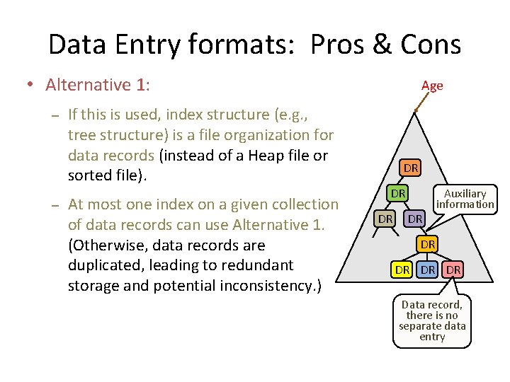
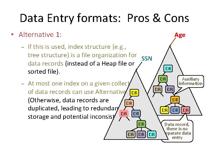
Data Entry formats: Pros & Cons • Alternative 1: – – Age If this is used, index structure (e. g. , tree structure) is a file organization for data records (instead of a Heap file or sorted file). At most one index on a given collection of data records can use Alternative 1. (Otherwise, data records are duplicated, leading to redundant storage and potential inconsistency. ) DR DR Auxiliary information DR DR Data record, there is no separate data entry

Data Entry formats: Pros & Cons • Alternative 1: – – Age If this is used, index structure (e. g. , tree structure) is a file organization for SSN data records (instead of a Heap file or sorted file). At most one index on a given collection of data records can use Alternative 1. DR (Otherwise, data records are DR duplicated, leading to redundant DR DR storage and potential inconsistency. ) DR DR Auxiliary information DR DR Data record, there is no separate data entry

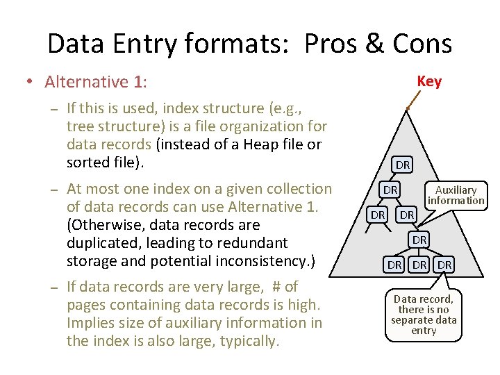
Data Entry formats: Pros & Cons • Alternative 1: – – – Key If this is used, index structure (e. g. , tree structure) is a file organization for data records (instead of a Heap file or sorted file). At most one index on a given collection of data records can use Alternative 1. (Otherwise, data records are duplicated, leading to redundant storage and potential inconsistency. ) If data records are very large, # of pages containing data records is high. Implies size of auxiliary information in the index is also large, typically. DR DR Auxiliary information DR DR Data record, there is no separate data entry

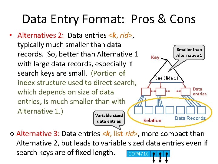
Data Entry Format: Pros & Cons • Alternatives 2: Data entries <k, rid>, typically much smaller than data records. So, better than Alternative 1 with large data records, especially if search keys are small. (Portion of index structure used to direct search, which depends on size of data entries, is much smaller than with Alternative 1. ) Variable sized data entries Key Smaller than Alternative 1 See Slide 11 Data entries Relation Data Records v Alternative 3: Data entries <k, list-rid>, more compact than Alternative 2, but leads to variable sized data entries even if search keys are of fixed length. COP 4710

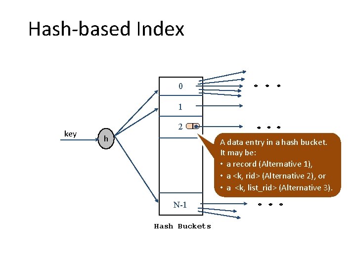
Hash-based Index 0 1 key 2 h A data entry in a hash bucket. It may be: • a record (Alternative 1), • a <k, rid> (Alternative 2), or • a <k, list_rid> (Alternative 3). N-1 Hash Buckets

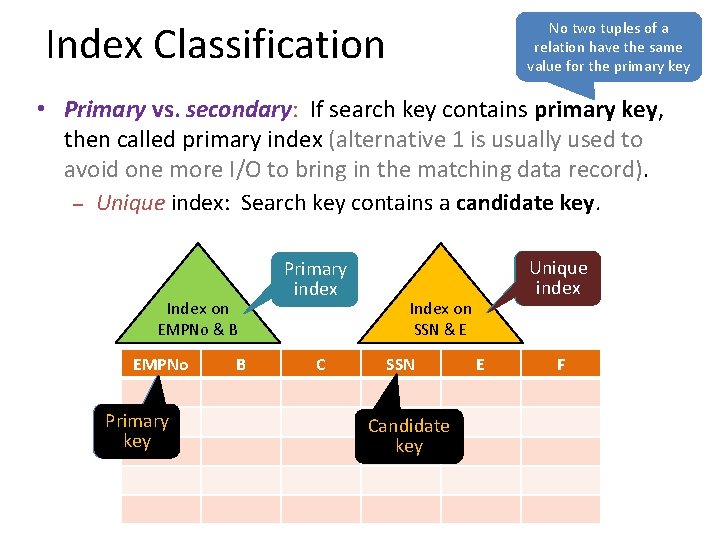
Index Classification No two tuples of a relation have the same value for the primary key • Primary vs. secondary: If search key contains primary key, then called primary index (alternative 1 is usually used to avoid one more I/O to bring in the matching data record). – Unique index: Search key contains a candidate key. Primary index Index on EMPNo & B EMPNo Primary key B Index on Unique index SSN & E C SSN Candidate key E F

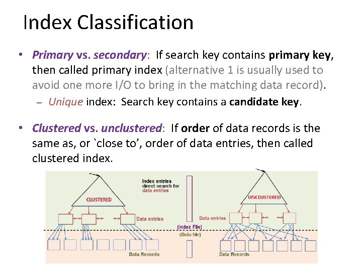
Index Classification • Primary vs. secondary: If search key contains primary key, then called primary index (alternative 1 is usually used to avoid one more I/O to bring in the matching data record). – Unique index: Search key contains a candidate key. • Clustered vs. unclustered: If order of data records is the same as, or `close to’, order of data entries, then called clustered index.

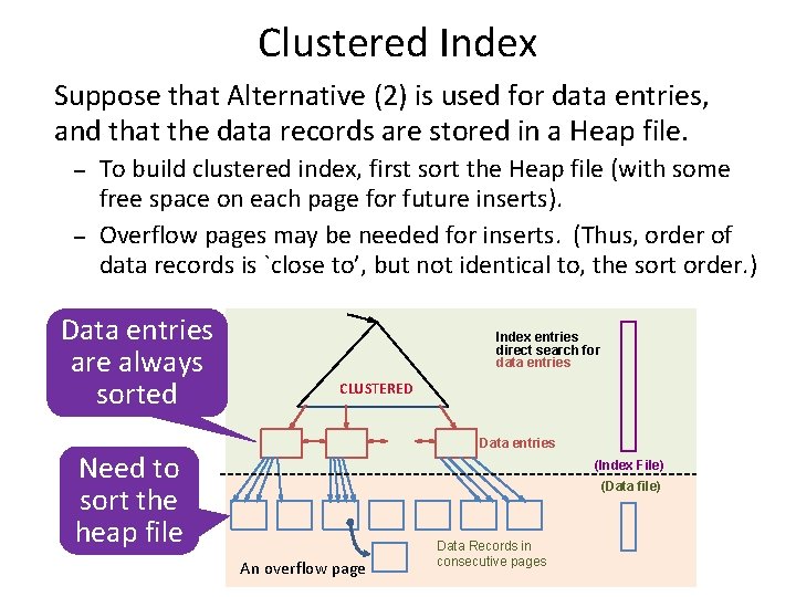
Clustered Index Suppose that Alternative (2) is used for data entries, and that the data records are stored in a Heap file. – – To build clustered index, first sort the Heap file (with some free space on each page for future inserts). Overflow pages may be needed for inserts. (Thus, order of data records is `close to’, but not identical to, the sort order. ) Data entries are always sorted Index entries direct search for data entries CLUSTERED Data entries Need to sort the heap file (Index File) (Data file) An overflow page Data Records in consecutive pages

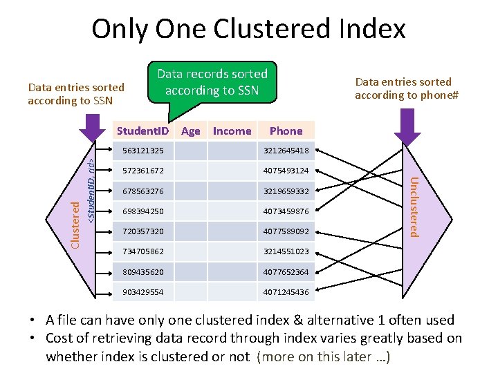
Only One Clustered Index Data entries sorted according to SSN Data records sorted according to SSN <Student. ID, rid> Income Phone 563121325 3212645418 572361672 4075493124 678563276 3219659332 698394250 4073459876 720357320 4077589092 734705862 3214551023 809435620 4077652364 903429554 4071245436 Unclustered Clustered Student. ID Age Data entries sorted according to phone# • A file can have only one clustered index & alternative 1 often used • Cost of retrieving data record through index varies greatly based on whether index is clustered or not (more on this later …)

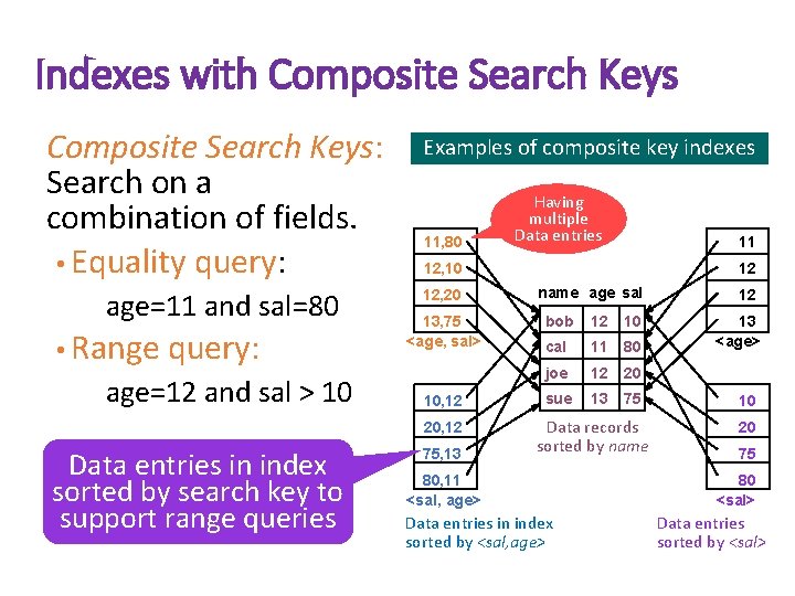
Indexes with Composite Search Keys: Search on a combination of fields. • Equality query: age=11 and sal=80 • Range query: age=12 and sal > 10 Examples of composite key indexes 11, 80 11 12, 10 12, 20 13, 75 <age, sal> 10, 12 20, 12 Data entries in index sorted by search key to support range queries Having multiple Data entries 75, 13 12 name age sal bob 12 10 cal 11 80 joe 12 20 sue 13 75 Data records sorted by name 80, 11 <sal, age> Data entries in index sorted by <sal, age> 12 13 <age> 10 20 75 80 <sal> Data entries sorted by <sal>

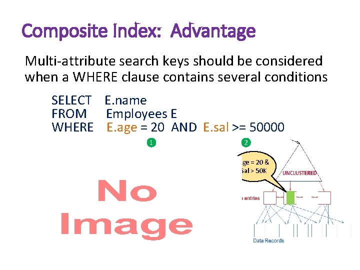
Composite Index: Advantage Multi-attribute search keys should be considered when a WHERE clause contains several conditions SELECT E. name FROM Employees E WHERE E. age = 20 AND E. sal >= 50000 1 2 Age = 20 & Sal > 50 K

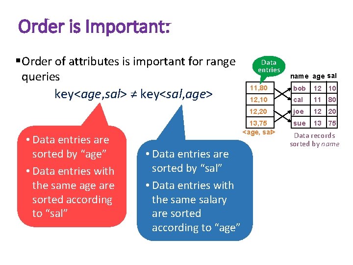
Order is Important: § Order of attributes is important for range queries key<age, sal> ≠ key<sal, age> • Data entries are sorted by “age” • Data entries with the same age are sorted according to “sal” • Data entries are sorted by “sal” • Data entries with the same salary are sorted according to “age” Data entries name age sal 11, 80 bob 12 10 12, 10 cal 11 80 12, 20 joe 12 20 13, 75 <age, sal> sue 13 75 Data records sorted by name

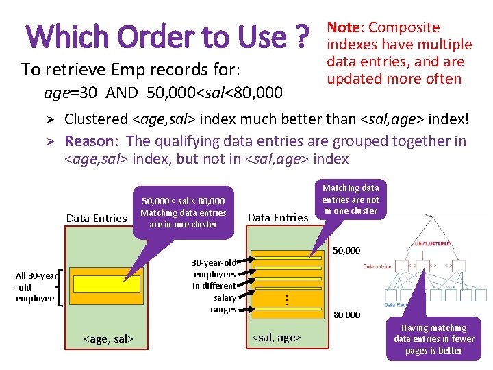
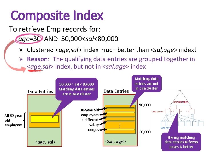
Which Order to Use ? To retrieve Emp records for: age=30 AND 50, 000<sal<80, 000 Ø Ø Note: Composite indexes have multiple data entries, and are updated more often Clustered <age, sal> index much better than <sal, age> index! Reason: The qualifying data entries are grouped together in <age, sal> index, but not in <sal, age> index Data Entries 50, 000 < sal < 80, 000 Matching data entries are in one cluster Data Entries Matching data entries are not in one cluster 50, 000 30 -year-old employees in different salary ranges All 30 -year -old employee <age, sal> . . . 80, 000 <sal, age> Having matching data entries in fewer pages is better

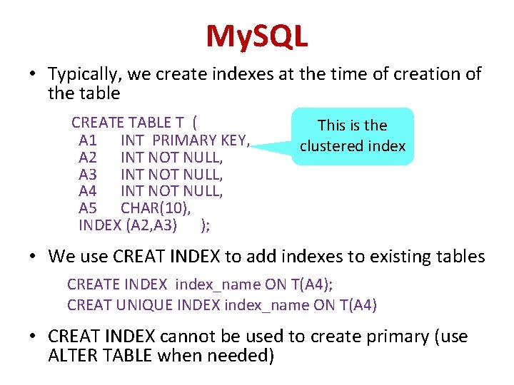
My. SQL • Typically, we create indexes at the time of creation of the table CREATE TABLE T ( This is the A 1 INT PRIMARY KEY, A 2 INT NOT NULL, A 3 INT NOT NULL, A 4 INT NOT NULL, A 5 CHAR(10), INDEX (A 2, A 3) ); clustered index • We use CREAT INDEX to add indexes to existing tables CREATE INDEX index_name ON T(A 4); CREAT UNIQUE INDEX index_name ON T(A 4) • CREAT INDEX cannot be used to create primary (use ALTER TABLE when needed)

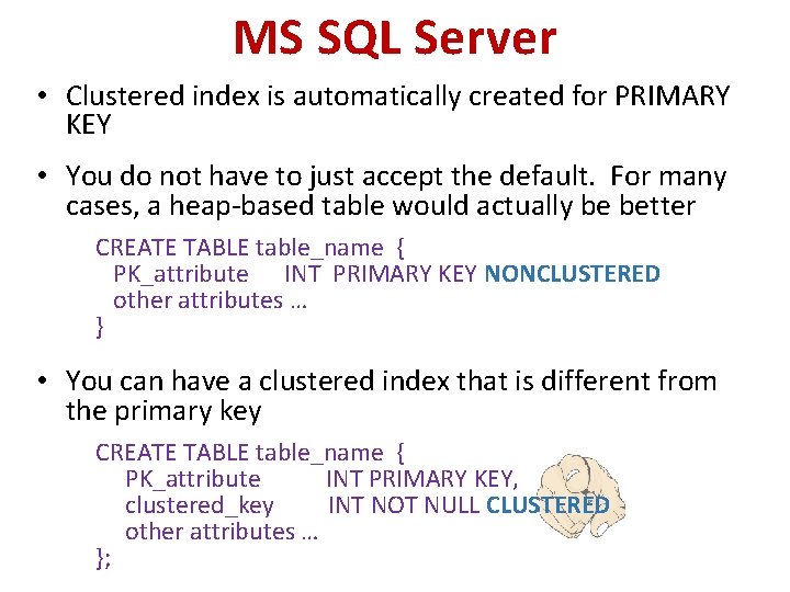
MS SQL Server • Clustered index is automatically created for PRIMARY KEY • You do not have to just accept the default. For many cases, a heap-based table would actually be better CREATE TABLE table_name { PK_attribute INT PRIMARY KEY NONCLUSTERED other attributes … } • You can have a clustered index that is different from the primary key CREATE TABLE table_name { PK_attribute INT PRIMARY KEY, clustered_key INT NOT NULL CLUSTERED other attributes … };

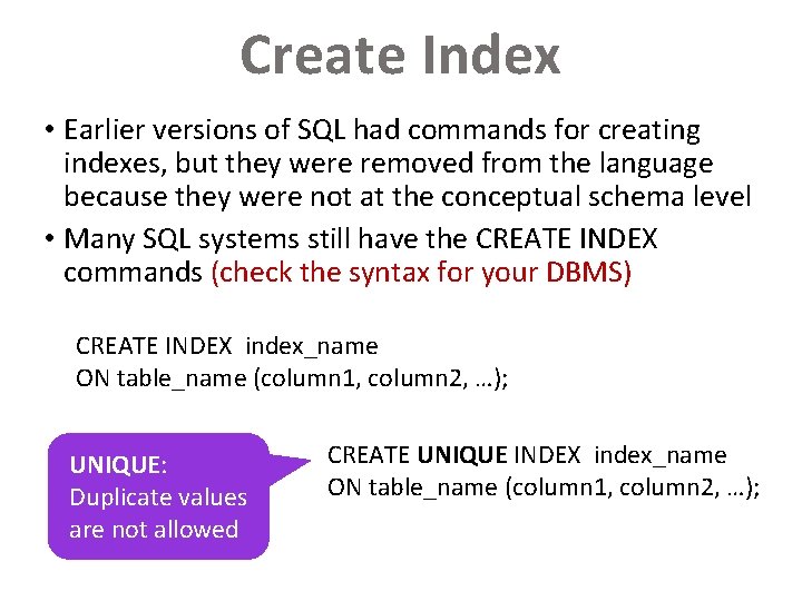
Create Index • Earlier versions of SQL had commands for creating indexes, but they were removed from the language because they were not at the conceptual schema level • Many SQL systems still have the CREATE INDEX commands (check the syntax for your DBMS) CREATE INDEX index_name ON table_name (column 1, column 2, …); UNIQUE: Duplicate values are not allowed CREATE UNIQUE INDEX index_name ON table_name (column 1, column 2, …);

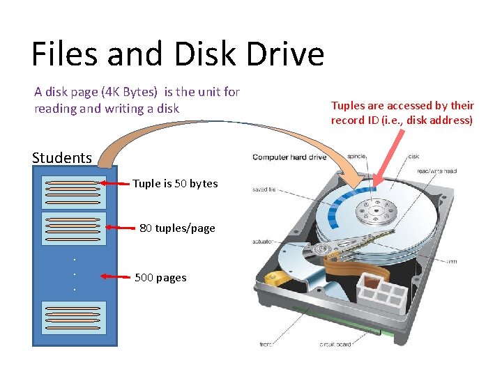
Files and Disk Drive A disk page (4 K Bytes) is the unit for reading and writing a disk Students Tuple is 50 bytes 80 tuples/page. . . 500 pages Tuples are accessed by their record ID (i. e. , disk address)

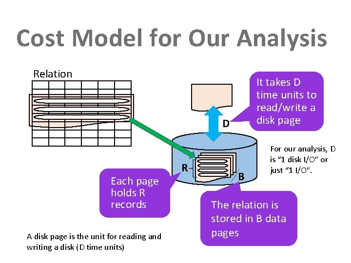
Cost Model for Our Analysis Relation It takes D time units to read/write a disk page D Each page holds R records A disk page is the unit for reading and writing a disk (D time units) R B For our analysis, D is “ 1 disk I/O” or just “ 1 I/O”. The relation is stored in B data pages

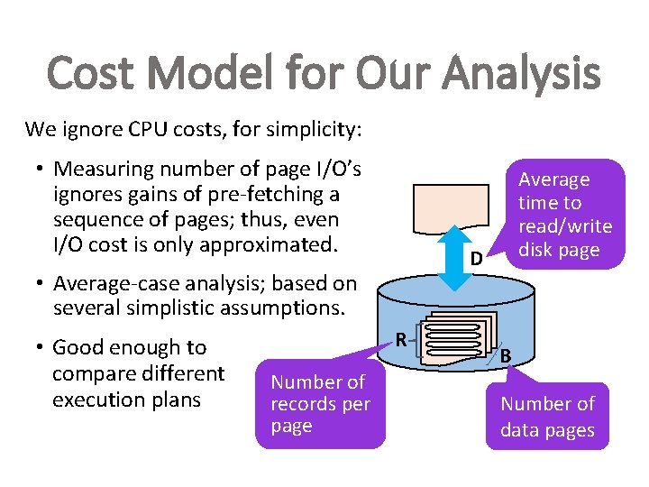
Cost Model for Our Analysis We ignore CPU costs, for simplicity: • Measuring number of page I/O’s ignores gains of pre-fetching a sequence of pages; thus, even I/O cost is only approximated. D • Average-case analysis; based on several simplistic assumptions. • Good enough to compare different execution plans R Number of records per page Average time to read/write disk page B Number of data pages

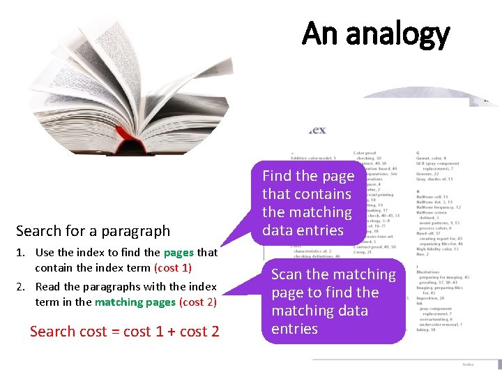
An analogy Search for a paragraph 1. Use the index to find the pages that contain the index term (cost 1) 2. Read the paragraphs with the index term in the matching pages (cost 2) Search cost = cost 1 + cost 2 Find the page that contains the matching data entries Scan the matching page to find the matching data entries

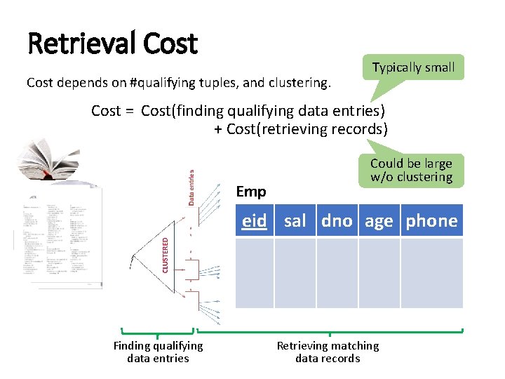
Retrieval Cost depends on #qualifying tuples, and clustering. Typically small Cost = Cost(finding qualifying data entries) + Cost(retrieving records) Emp Could be large w/o clustering eid sal dno age phone Finding qualifying data entries Retrieving matching data records

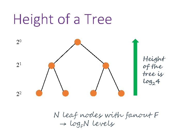
Height of a Tree 20 21 Height of the tree is log 24 22 N leaf nodes with fanout F → log. FN levels

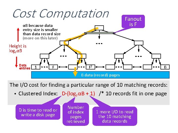
Cost Computation αB because data entry size is smaller than data record size (more on this later) Fanout is F Height is log. FαB Data entries 1 F F 2 B B data (record) pages The I/O cost for finding a particular range of 10 matching records: § Clustered Index: D (log. FαB + 1) /* 10 records fit in one page D is time to read or write a disk page Number of index pages retrieved 1 more I/O to read the 10 matching data records

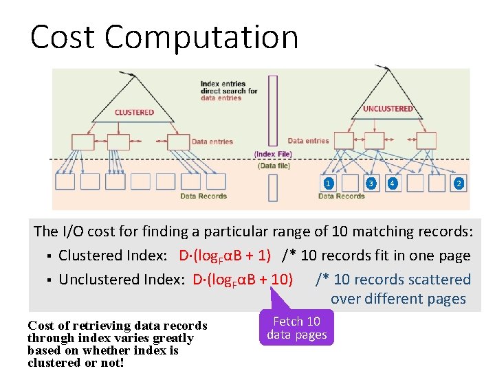
Cost Computation 1 3 4 2 The I/O cost for finding a particular range of 10 matching records: § Clustered Index: D (log. FαB + 1) /* 10 records fit in one page § Unclustered Index: D (log. FαB + 10) /* 10 records scattered over different pages Cost of retrieving data records through index varies greatly based on whether index is clustered or not! Fetch 10 data pages

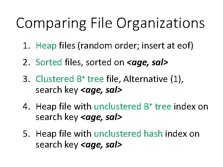
Comparing File Organizations 1. Heap files (random order; insert at eof) 2. Sorted files, sorted on <age, sal> 3. Clustered B+ tree file, Alternative (1), search key <age, sal> 4. Heap file with unclustered B+ tree index on search key <age, sal> 5. Heap file with unclustered hash index on search key <age, sal>

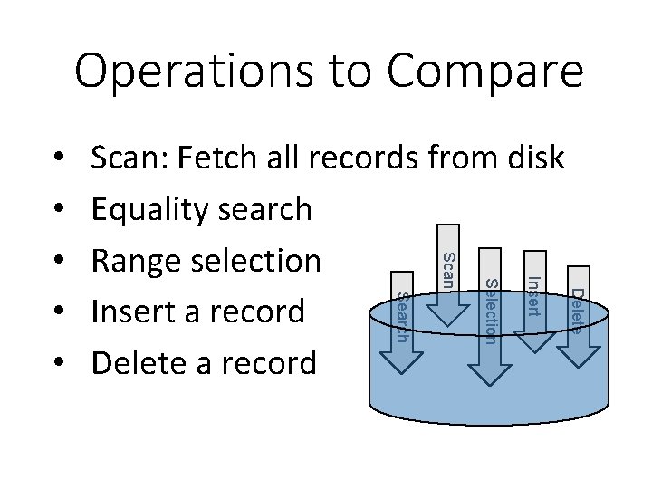
Operations to Compare Delete Insert Selection Scan: Fetch all records from disk Equality search Range selection Insert a record Delete a record Search • • •

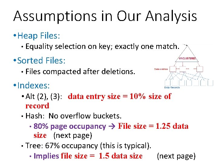
Assumptions in Our Analysis • Heap Files: • Equality selection on key; exactly one match. • Sorted Files: • Files compacted after deletions. • Indexes: • Alt (2), (3): data entry size = 10% size of record • Hash: No overflow buckets. • 80% page occupancy → File size = 1. 25 data size (next page) • Tree: 67% occupancy (this is typical). • Implies file size = 1. 5 data size (next page)

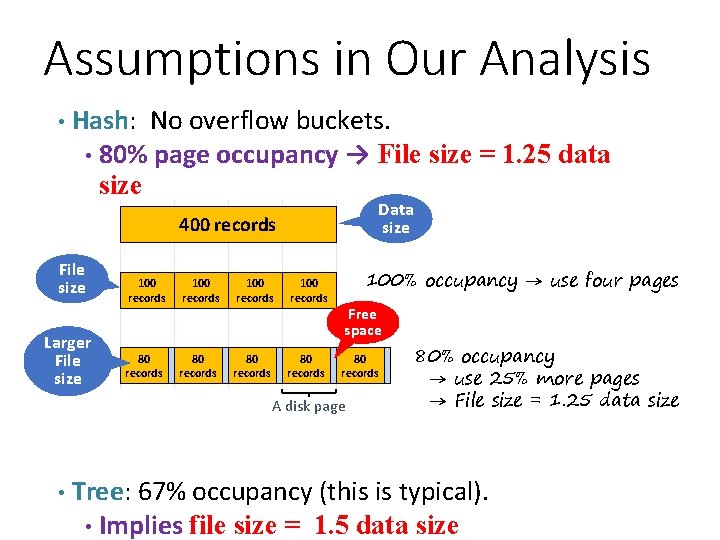
Assumptions in Our Analysis • Hash: No overflow buckets. • 80% page occupancy → size Data size 400 records File size Larger File size = 1. 25 data 100 records 80 records 100% occupancy → use four pages Free space 80 records A disk page 80% occupancy → use 25% more pages → File size = 1. 25 data size • Tree: 67% occupancy (this is typical). • Implies file size = 1. 5 data size

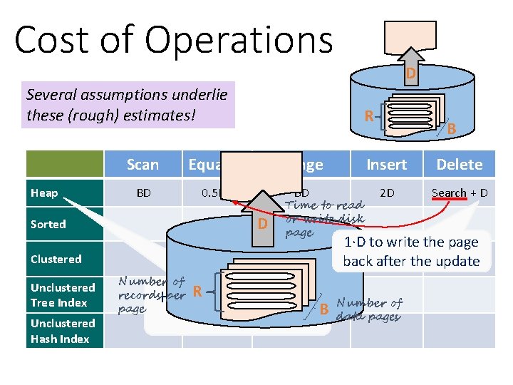
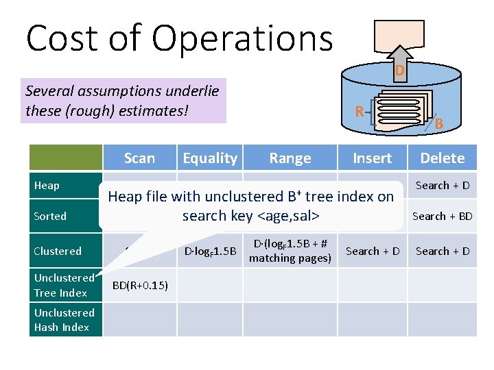
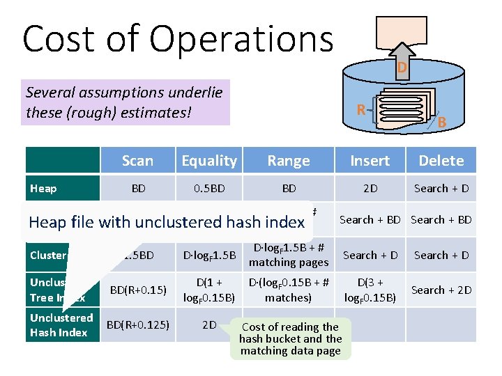
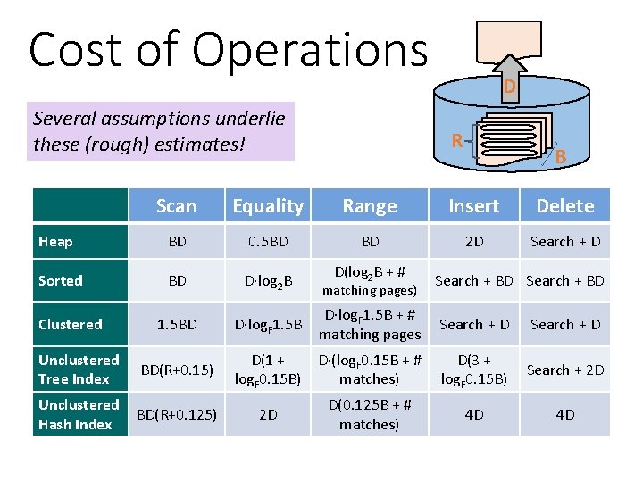
Cost of Operations Several assumptions underlie these (rough) estimates! Heap Sorted Clustered Unclustered Tree Index Unclustered Hash Index D R B Scan Equality Range Insert Delete BD 0. 5 BD BD 2 D Search + D D Time to read or write disk page 1·D to write the page back after the update Number of records. Heap files (not sorted; per R Number of page B data pages insert at eof)

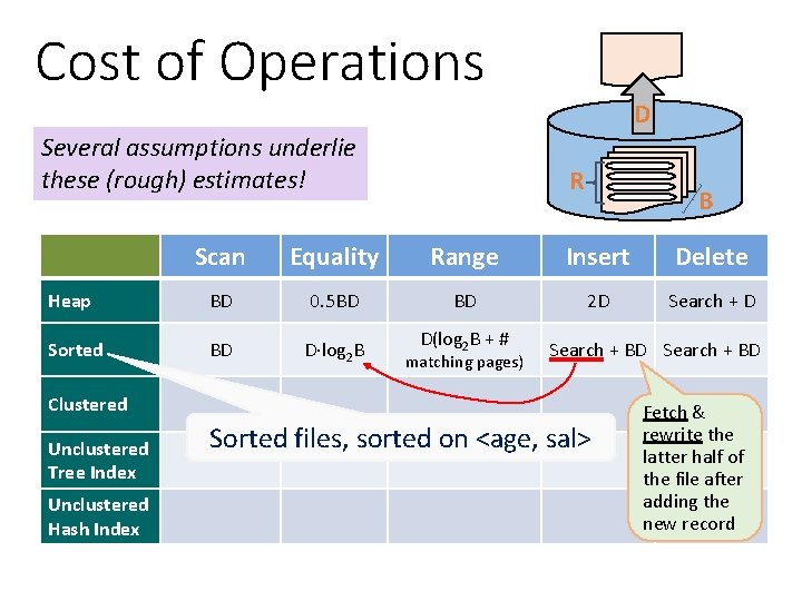
Cost of Operations D Several assumptions underlie these (rough) estimates! R B Scan Equality Range Insert Delete Heap BD 0. 5 BD BD 2 D Search + D Sorted BD D log 2 B D(log 2 B + # matching pages) Search + BD Clustered Unclustered Tree Index Unclustered Hash Index Sorted files, sorted on <age, sal> Fetch & rewrite the latter half of the file after adding the new record

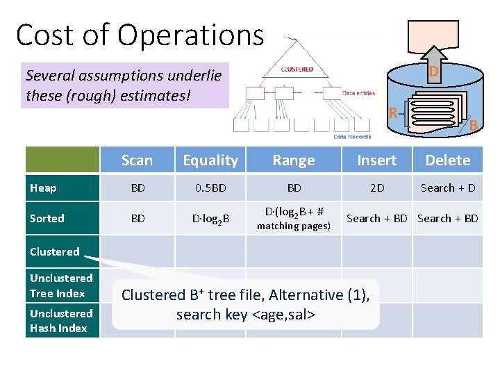
Cost of Operations D Several assumptions underlie these (rough) estimates! R B Scan Equality Range Insert Delete Heap BD 0. 5 BD BD 2 D Search + D Sorted BD D log 2 B D (log 2 B + # matching pages) Search + BD Clustered Unclustered Tree Index Unclustered Hash Index Clustered B+ tree file, Alternative (1), search key <age, sal>

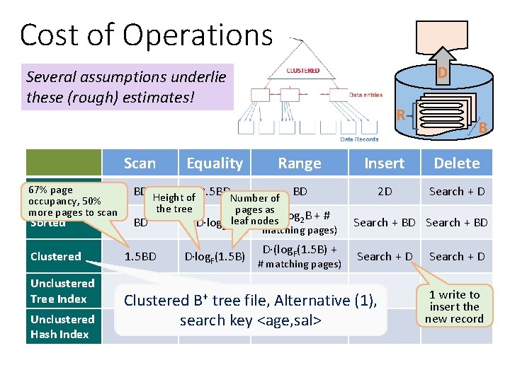
Cost of Operations D Several assumptions underlie these (rough) estimates! Scan 67% page Heap occupancy, 50% more pages to scan Sorted Clustered Unclustered Tree Index Unclustered Hash Index Equality R Range BD Height of 0. 5 BD BD Number of the tree pages as D (log 2 B + # BD D log 2 Bleaf nodes matching pages) 1. 5 BD D log. F(1. 5 B) D (log. F(1. 5 B) + # matching pages) B Insert Delete 2 D Search + BD Search + D Clustered B+ tree file, Alternative (1), search key <age, sal> Search + D 1 write to insert the new record

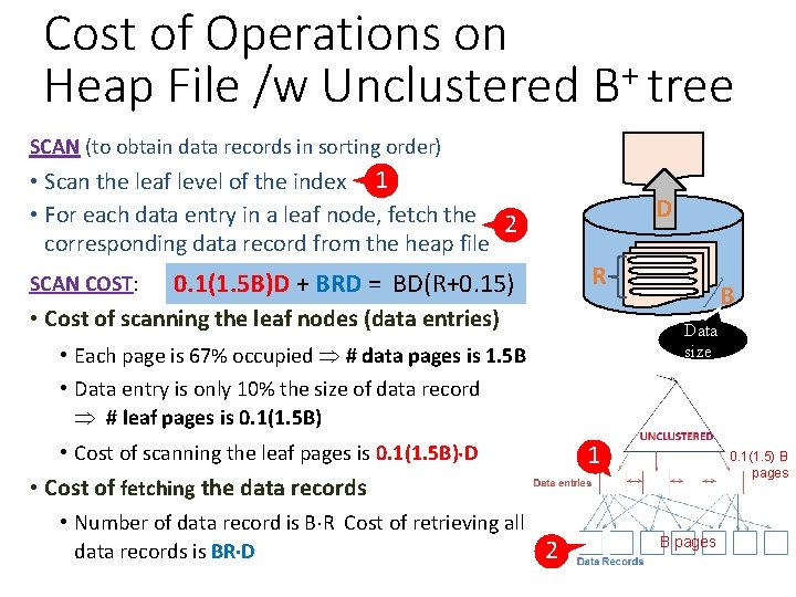
Cost of Operations on + Heap File /w Unclustered B tree SCAN (to obtain data records in sorting order) • Scan the leaf level of the index 1 • For each data entry in a leaf node, fetch the 2 corresponding data record from the heap file SCAN COST: 0. 1(1. 5 B)D + BRD = BD(R+0. 15) D R • Cost of scanning the leaf nodes (data entries) Data size • Each page is 67% occupied # data pages is 1. 5 B • Data entry is only 10% the size of data record # leaf pages is 0. 1(1. 5 B) • Cost of scanning the leaf pages is 0. 1(1. 5 B) D B 1 0. 1(1. 5) B pages • Cost of fetching the data records • Number of data record is B R Cost of retrieving all data records is BR D 2 B pages

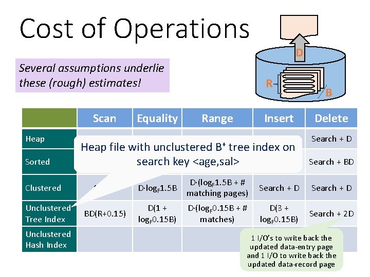
Cost of Operations Several assumptions underlie these (rough) estimates! Heap Sorted Clustered Unclustered Tree Index Unclustered Hash Index D R B Scan Equality Range Insert Delete BD 0. 5 BD BD 2 D Search + D Heap file with unclustered B+ tree index on BD 1. 5 BD BD(R+0. 15) D (log B + # 2 D log 2 B search key <age, sal> matches) D log. F 1. 5 B D (log. F 1. 5 B + # matching pages) Search + BD Search + D

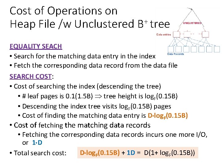
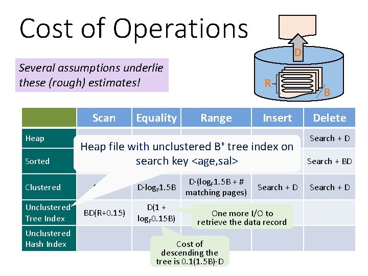
Cost of Operations on Heap File /w Unclustered B+ tree EQUALITY SEACH • Search for the matching data entry in the index • Fetch the corresponding data record from the data file SEARCH COST: • Cost of searching the index (descending the tree) • # leaf pages is 0. 1(1. 5 B) tree height is log. F(0. 15 B) • Descending the index tree visits log. F(0. 15 B) pages • Cost of finding the matching data entry is D log. F(0. 15 B) • Cost of fetching the matching data records • Fetching the corresponding data records incurs one more I/O, or 1 D • Total search cost: D log. F(0. 15 B) + 1 D = D(1+ log. F(0. 15 B))

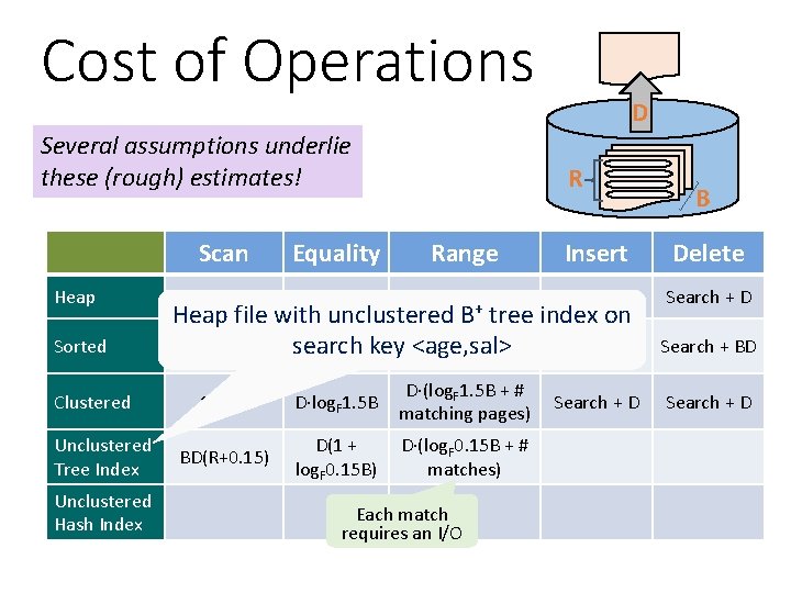
Cost of Operations Several assumptions underlie these (rough) estimates! Heap Sorted Clustered Unclustered Tree Index Unclustered Hash Index D R B Scan Equality Range Insert Delete BD 0. 5 BD BD 2 D Search + D Heap file with unclustered B+ tree index on BD D (log B + # 2 D log 2 B search key <age, sal> matches) 1. 5 BD D log. F 1. 5 B BD(R+0. 15) D(1 + log. F 0. 15 B) D (log. F 1. 5 B + # matching pages) Search + BD Search + D One more I/O to retrieve the data record Cost of descending the tree is 0. 1(1. 5 B) D Search + D

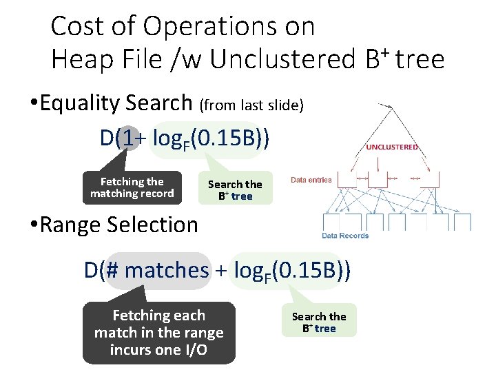
Cost of Operations on Heap File /w Unclustered B+ tree • Equality Search (from last slide) D(1+ log. F(0. 15 B)) Fetching the matching record Search the B+ tree • Range Selection D(# matches + log. F(0. 15 B)) Fetching each match in the range incurs one I/O Search the B+ tree

Cost of Operations Several assumptions underlie these (rough) estimates! Heap Sorted Clustered Unclustered Tree Index Unclustered Hash Index D R B Scan Equality Range Insert Delete BD 0. 5 BD BD 2 D Search + D Heap file with unclustered B+ tree index on BD D (log B + # 2 D log 2 B search key <age, sal> matches) 1. 5 BD D log. F 1. 5 B D (log. F 1. 5 B + # matching pages) BD(R+0. 15) D(1 + log. F 0. 15 B) D (log. F 0. 15 B + # matches) Each match requires an I/O Search + BD Search + D

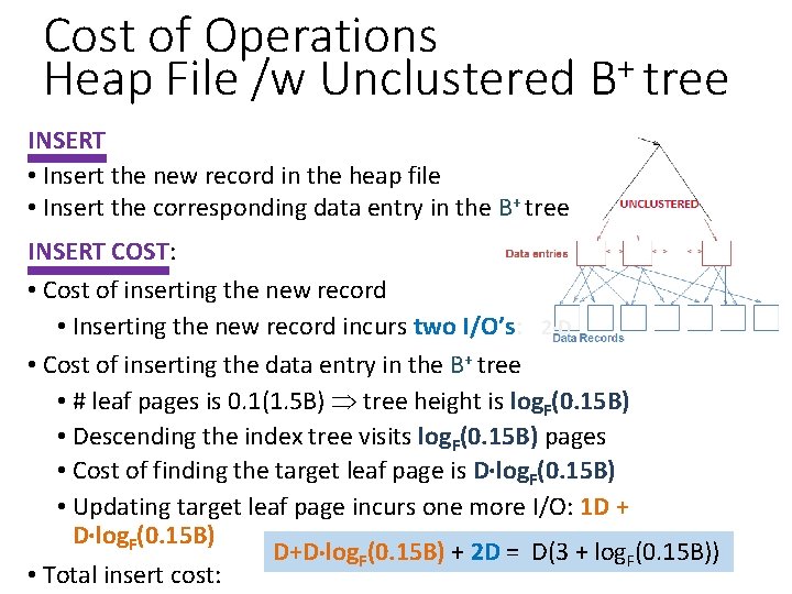
Cost of Operations + Heap File /w Unclustered B tree INSERT • Insert the new record in the heap file • Insert the corresponding data entry in the B+ tree INSERT COST: • Cost of inserting the new record • Inserting the new record incurs two I/O’s: 2 D • Cost of inserting the data entry in the B+ tree • # leaf pages is 0. 1(1. 5 B) tree height is log. F(0. 15 B) • Descending the index tree visits log. F(0. 15 B) pages • Cost of finding the target leaf page is D log. F(0. 15 B) • Updating target leaf page incurs one more I/O: 1 D + D log. F(0. 15 B) D+D log. F(0. 15 B) + 2 D = D(3 + log. F(0. 15 B)) • Total insert cost:

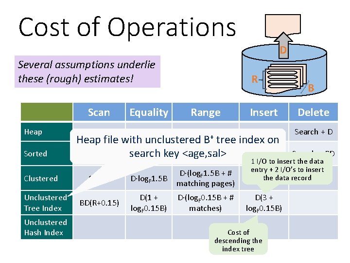
Cost of Operations Several assumptions underlie these (rough) estimates! Heap Sorted Clustered Unclustered Tree Index Unclustered Hash Index D R B Scan Equality Range Insert Delete BD 0. 5 BD BD 2 D Search + D Heap file with unclustered B+ tree index on BD D (log B + # 2 D log 2 B search key <age, sal> matches) 1. 5 BD D log. F 1. 5 B D (log. F 1. 5 B + # matching pages) BD(R+0. 15) D(1 + log. F 0. 15 B) D (log. F 0. 15 B + # matches) Search + BD 1 I/O to insert the data entry + 2 I/O’s to insert the data record Search + D D(3 + log. F 0. 15 B) Cost of descending the index tree

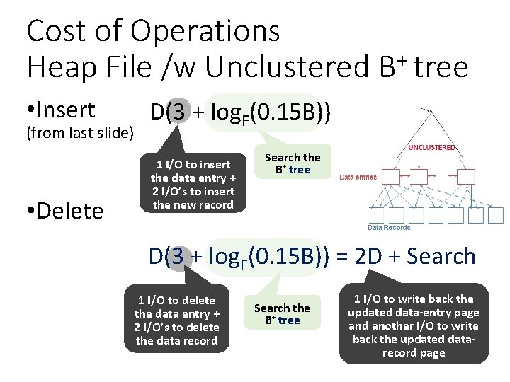
Cost of Operations + Heap File /w Unclustered B tree • Insert (from last slide) • Delete D(3 + log. F(0. 15 B)) 1 I/O to insert the data entry + 2 I/O’s to insert the new record Search the B+ tree D(3 + log. F(0. 15 B)) = 2 D + Search 1 I/O to delete the data entry + 2 I/O’s to delete the data record Search the B+ tree 1 I/O to write back the updated data-entry page and another I/O to write back the updated datarecord page

Cost of Operations Several assumptions underlie these (rough) estimates! Heap Sorted Clustered Unclustered Tree Index Unclustered Hash Index D R B Scan Equality Range Insert Delete BD 0. 5 BD BD 2 D Search + D Heap file with unclustered B+ tree index on BD D (log B + # 2 D log 2 B search key <age, sal> matches) Search + BD 1. 5 BD D log. F 1. 5 B D (log. F 1. 5 B + # matching pages) Search + D BD(R+0. 15) D(1 + log. F 0. 15 B) D (log. F 0. 15 B + # matches) D(3 + log. F 0. 15 B) Search + 2 D 1 I/O’s to write back the updated data-entry page and 1 I/O to write back the updated data-record page

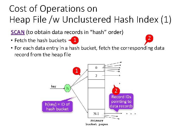
Cost of Operations on Heap File /w Unclustered Hash Index (1) SCAN (to obtain data records in “hash” order) • Fetch the hash buckets 1 2 • For each data entry in a hash bucket, fetch the corresponding data record from the heap file 1 2

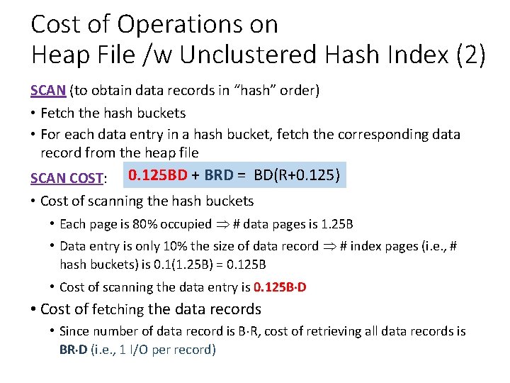
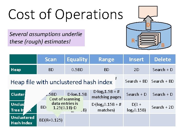
Cost of Operations on Heap File /w Unclustered Hash Index (2) SCAN (to obtain data records in “hash” order) • Fetch the hash buckets • For each data entry in a hash bucket, fetch the corresponding data record from the heap file SCAN COST: 0. 125 BD + BRD = BD(R+0. 125) • Cost of scanning the hash buckets • Each page is 80% occupied # data pages is 1. 25 B • Data entry is only 10% the size of data record # index pages (i. e. , # hash buckets) is 0. 1(1. 25 B) = 0. 125 B • Cost of scanning the data entry is 0. 125 B D • Cost of fetching the data records • Since number of data record is B R, cost of retrieving all data records is BR D (i. e. , 1 I/O per record)

Cost of Operations Several assumptions underlie these (rough) estimates! Heap R Unclustered Tree Index Unclustered Hash Index B Scan Equality Range Insert Delete BD 0. 5 BD BD 2 D Search + D D(log 2 B + # Sorted BD D log B 2 Heap file with unclustered hash index matches) Clustered D Search + BD D log. F 1. 5 B + # 1. 5 BD D log. F 1. 5 B Search + D matching pages Cost of scanning data entries is D(1 + D (log. F 0. 15 B + # D(3 + BD(R+0. 15) 1. 25(0. 1 B) D log. F 0. 15 B) matches) log. F 0. 15 B) BD(R+0. 125) Search + D Search + 2 D

Cost of Operations D Several assumptions underlie these (rough) estimates! Heap R B Scan Equality Range Insert Delete BD 0. 5 BD BD 2 D Search + D D(log 2 B + # Sorted BD D log B 2 Heap file with unclustered hash index matches) Search + BD 1. 5 BD D log. F 1. 5 B + # matching pages Search + D Unclustered Tree Index BD(R+0. 15) D(1 + log. F 0. 15 B) D (log. F 0. 15 B + # D(3 + matches) log. F 0. 15 B) Search + 2 D Unclustered Hash Index BD(R+0. 125) 2 D Clustered Cost of reading the hash bucket and the matching data page

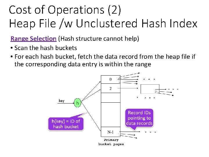
Cost of Operations (2) Heap File /w Unclustered Hash Index Range Selection (Hash structure cannot help) • Scan the hash buckets • For each hash bucket, fetch the data record from the heap file if the corresponding data entry is within the range

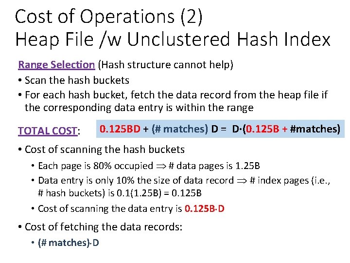
Cost of Operations (2) Heap File /w Unclustered Hash Index Range Selection (Hash structure cannot help) • Scan the hash buckets • For each hash bucket, fetch the data record from the heap file if the corresponding data entry is within the range TOTAL COST: 0. 125 BD + (# matches) D = D∙(0. 125 B + #matches) • Cost of scanning the hash buckets • Each page is 80% occupied # data pages is 1. 25 B • Data entry is only 10% the size of data record # index pages (i. e. , # hash buckets) is 0. 1(1. 25 B) = 0. 125 B • Cost of scanning the data entry is 0. 125 B D • Cost of fetching the data records: • (# matches) D

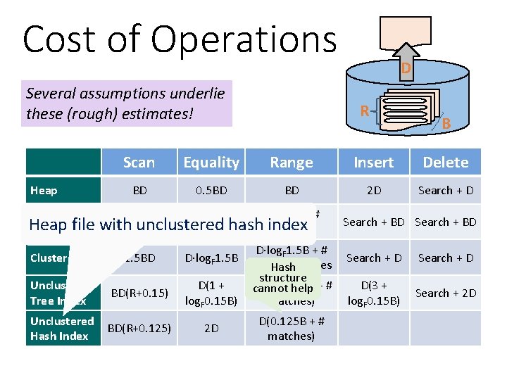
Cost of Operations Several assumptions underlie these (rough) estimates! Heap R B Scan Equality Range Insert Delete BD 0. 5 BD BD 2 D Search + D D(log 2 B + # Sorted BD D log B 2 Heap file with unclustered hash index matches) Clustered D 1. 5 BD D log. F 1. 5 B Unclustered Tree Index BD(R+0. 15) D(1 + log. F 0. 15 B) Unclustered Hash Index BD(R+0. 125) 2 D Search + BD D log. F 1. 5 B + # Search + D matching pages Hash structure D (log D(3 + cannot help F 0. 15 B + # matches) log. F 0. 15 B) D(0. 125 B + # matches) Search + D Search + 2 D

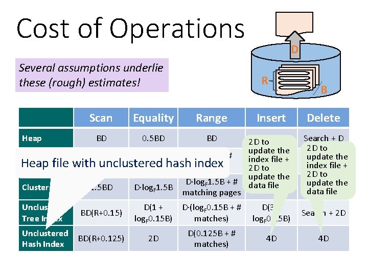
Cost of Operations Several assumptions underlie these (rough) estimates! R Scan Equality Range BD 0. 5 BD BD Unclustered Tree Index BD(R+0. 15) D(1 + log. F 0. 15 B) Unclustered Hash Index BD(R+0. 125) 2 D Heap D Insert B Delete 2 D Search + D 2 D to update the D(log 2 B + # update the index file + Sorted BD D log B Search + BD 2 Heap file with unclustered hash index file + matches) 2 D to update the D log. F 1. 5 B + # data file update the Clustered 1. 5 BD D log. F 1. 5 B Search + D data file matching pages D (log. F 0. 15 B + # D(3 + matches) log. F 0. 15 B) D(0. 125 B + # matches) 4 D Search + 2 D 4 D

Cost of Operations Several assumptions underlie these (rough) estimates! D R B Scan Equality Range Insert Delete Heap BD 0. 5 BD BD 2 D Search + D Sorted BD D log 2 B matching pages) 1. 5 BD D log. F 1. 5 B + # matching pages Search + D Unclustered Tree Index BD(R+0. 15) D(1 + log. F 0. 15 B) D (log. F 0. 15 B + # D(3 + matches) log. F 0. 15 B) Search + 2 D Unclustered Hash Index BD(R+0. 125) 2 D Clustered D(log 2 B + # D(0. 125 B + # matches) Search + BD 4 D 4 D

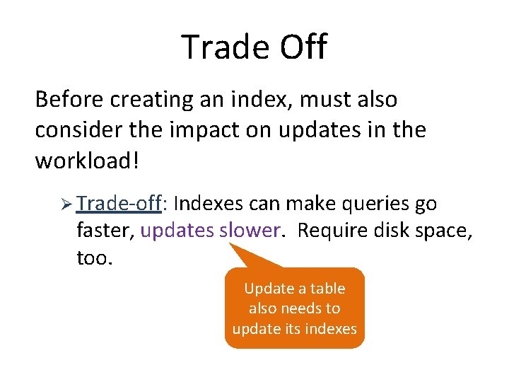
Trade Off Before creating an index, must also consider the impact on updates in the workload! Ø Trade-off: Indexes can make queries go faster, updates slower. Require disk space, too. Update a table also needs to update its indexes

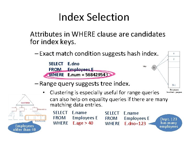
Index Selection Attributes in WHERE clause are candidates for index keys. – Exact match condition suggests hash index. SELECT E. dno FROM Employees E WHERE E. num = 568429543 – Range query suggests tree index. • Clustering is especially useful for range queries • can also help on equality queries if there are many matching data entries. Employees older than 40 SELECT E. name FROM Employees E WHERE E. age > 40 SELECT E. name FROM Employees E WHERE E. dno=123 Dept. 123 has many employees

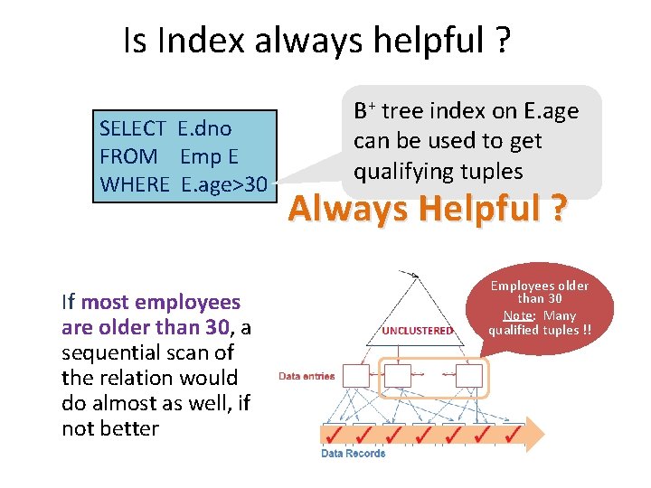
Is Index always helpful ? SELECT E. dno FROM Emp E WHERE E. age>30 If most employees are older than 30, a sequential scan of the relation would do almost as well, if not better B+ tree index on E. age can be used to get qualifying tuples Always Helpful ? Employees older than 30 Note: Many qualified tuples !!

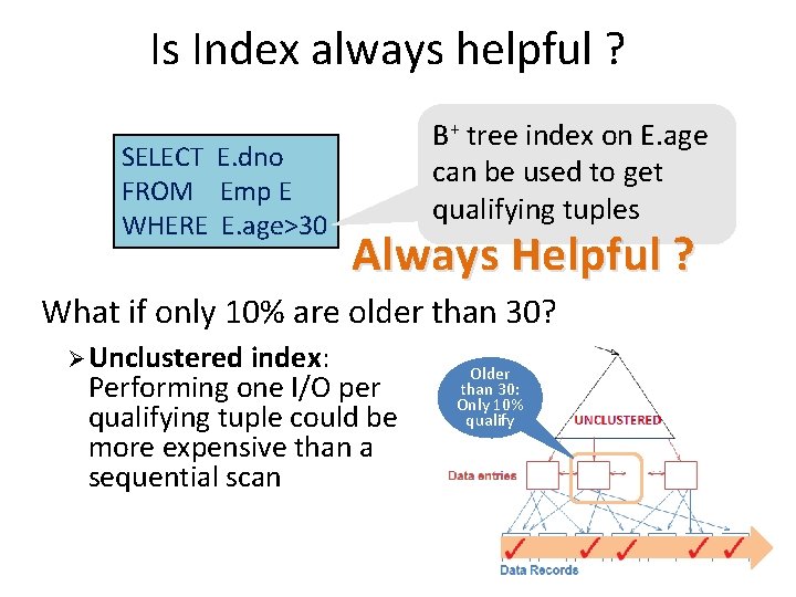
Is Index always helpful ? SELECT E. dno FROM Emp E WHERE E. age>30 B+ tree index on E. age can be used to get qualifying tuples Always Helpful ? What if only 10% are older than 30? Ø Unclustered index: Performing one I/O per qualifying tuple could be more expensive than a sequential scan Older than 30: Only 10% qualify

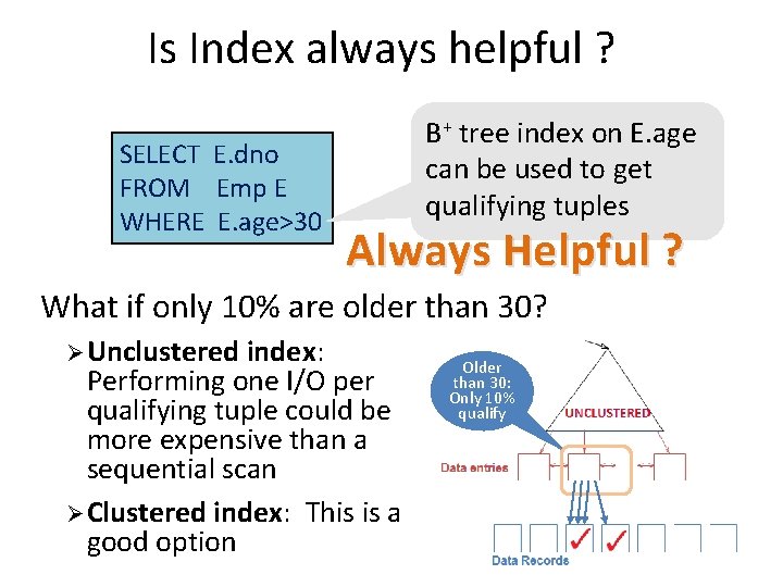
Is Index always helpful ? SELECT E. dno FROM Emp E WHERE E. age>30 B+ tree index on E. age can be used to get qualifying tuples Always Helpful ? What if only 10% are older than 30? Ø Unclustered index: Performing one I/O per qualifying tuple could be more expensive than a sequential scan Ø Clustered index: This is a good option Older than 30: Only 10% qualify

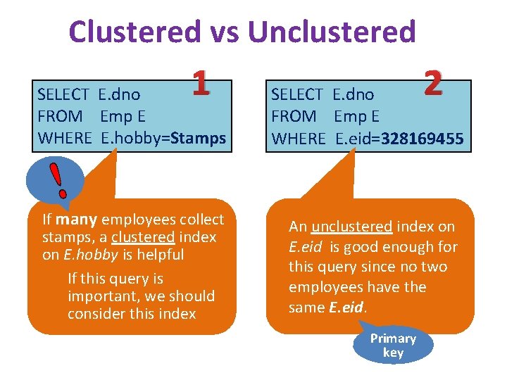
Clustered vs Unclustered 1 2 SELECT E. dno FROM Emp E WHERE E. hobby=Stamps SELECT E. dno FROM Emp E WHERE E. eid=328169455 If many employees collect stamps, a clustered index on E. hobby is helpful If this query is important, we should consider this index An unclustered index on E. eid is good enough for this query since no two employees have the same E. eid. Primary key

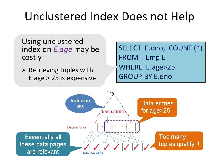
Unclustered Index Does not Help Using unclustered index on E. age may be costly Ø Retrieving tuples with E. age > 25 is expensive Index on age Essentially all these data pages are relevant SELECT E. dno, COUNT (*) FROM Emp E WHERE E. age>25 GROUP BY E. dno Data entries for age>25 Too many tuples qualify !!

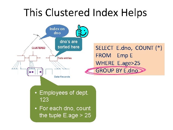
This Clustered Index Helps Index on dno’s are sorted here • Employees of dept. 123 • For each dno, count the tuple E. age > 25 SELECT E. dno, COUNT (*) FROM Emp E WHERE E. age>25 GROUP BY E. dno

Composite Index To retrieve Emp records for: age=30 AND 50, 000<sal<80, 000 Ø Ø Clustered <age, sal> index much better than <sal, age> index! Reason: The qualifying data entries are grouped together in <age, sal> index, but not in <sal, age> index Data Entries 50, 000 < sal < 80, 000 Matching data entries are in one cluster Data Entries Matching data entries are not in one cluster 50, 000 30 -year-old employees in different salary ranges All 30 -yearold employees <age, sal> . . . 80, 000 <sal, age> Having matching data entries in fewer pages is better

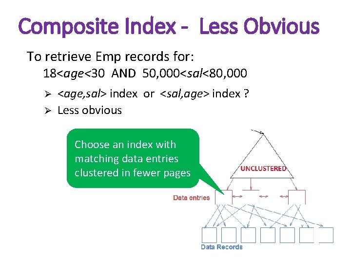
Composite Index - Less Obvious To retrieve Emp records for: 18<age<30 AND 50, 000<sal<80, 000 Ø Ø <age, sal> index or <sal, age> index ? Less obvious Choose an index with matching data entries clustered in fewer pages

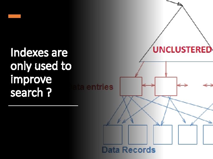
Indexes are only used to improve search ?

Index can be used to support indexonly evaluation

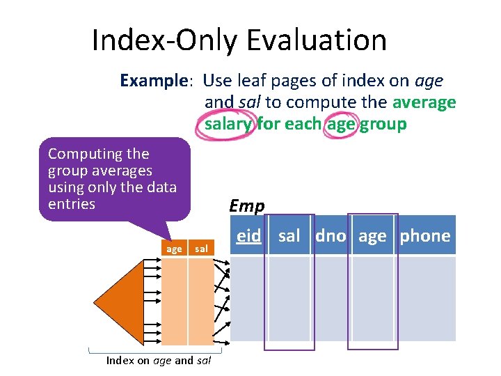
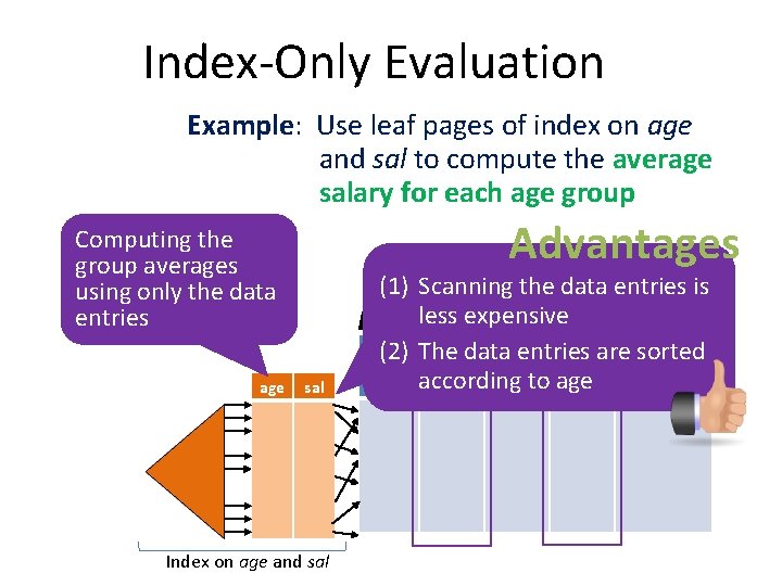
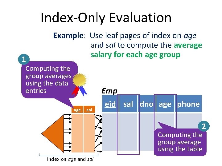
Index-Only Evaluation Example: Use leaf pages of index on age and sal to compute the average salary for each age group These data entries can be used as the two columns of the table Emp age Emp sal Index on age and sal eid sal dno age phone

Index-Only Evaluation Example: Use leaf pages of index on age and sal to compute the average salary for each age group Computing the group averages using only the data entries age Emp sal Index on age and sal eid sal dno age phone

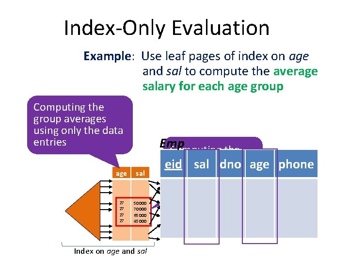
Index-Only Evaluation Example: Use leaf pages of index on age and sal to compute the average salary for each age group Computing the group averages using only the data entries Emp Computing the age sal 27 27 50000 70000 65000 45000 Index on age and sal average for the 27 eid sal dno age phone -year-old group

Index-Only Evaluation Example: Use leaf pages of index on age and sal to compute the average salary for each age group Advantages Computing the group averages using only the data entries age sal Index on age and sal (1) Scanning the data entries is Emp less expensive (2) The data entries are sorted eid according to age sal dno age phone

Index-Only Evaluation 1 Example: Use leaf pages of index on age and sal to compute the average salary for each age group Computing the group averages using the data entries Emp age sal eid sal dno age phone 2 Computing the group average using the table Index on age and sal

Index can be used to support indexonly evaluation Good to know DBMS internal

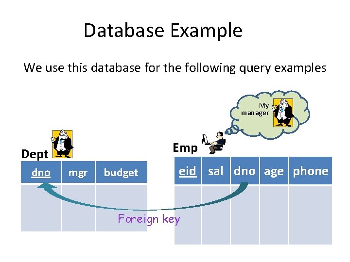
Database Example We use this database for the following query examples My manager Emp Dept dno mgr budget eid sal dno age phone Foreign key

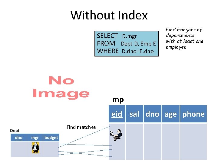
Without Index SELECT D. mgr FROM Dept D, Emp E WHERE D. dno=E. dno Find mangers of departments with at least one employee Emp eid sal dno age phone Find matches

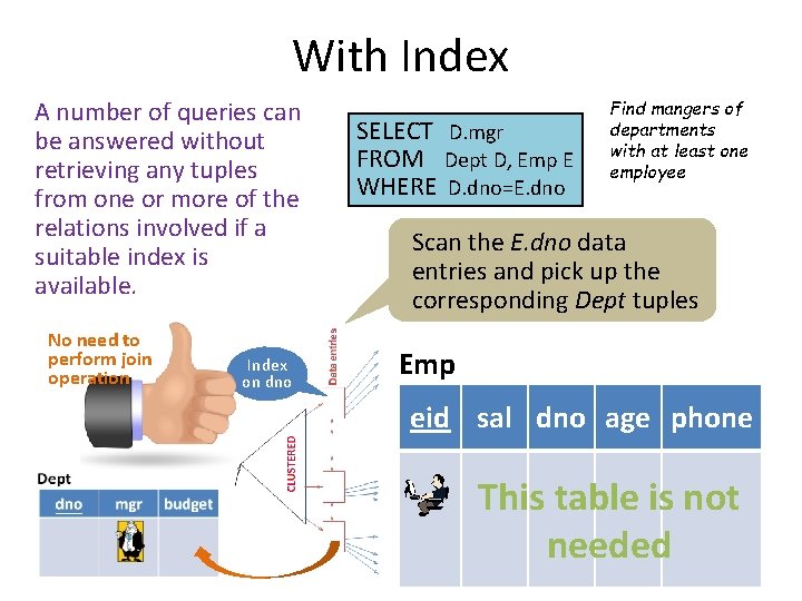
With Index A number of queries can be answered without retrieving any tuples from one or more of the relations involved if a suitable index is available. No need to perform join operation Index on dno SELECT D. mgr FROM Dept D, Emp E WHERE D. dno=E. dno Find mangers of departments with at least one employee Scan the E. dno data entries and pick up the corresponding Dept tuples Emp eid sal dno age phone This table is not needed

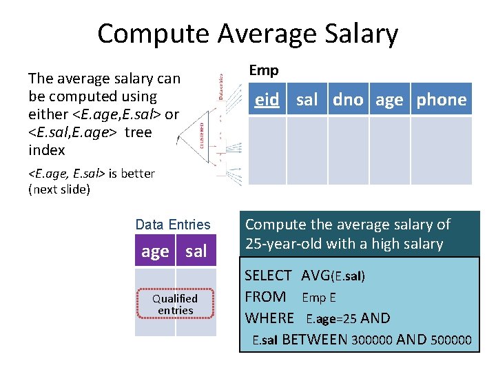
Compute Average Salary The average salary can be computed using either <E. age, E. sal> or <E. sal, E. age> tree index Emp eid sal dno age phone <E. age, E. sal> is better (next slide) Data Entries age sal Qualified entries Compute the average salary of 25 -year-old with a high salary SELECT AVG(E. sal) FROM Emp E WHERE E. age=25 AND E. sal BETWEEN 300000 AND 500000

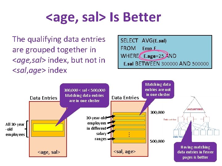
<age, sal> Is Better The qualifying data entries are grouped together in <age, sal> index, but not in <sal, age> index Data Entries 300, 000 < sal < 500, 000 Matching data entries are in one cluster SELECT AVG(E. sal) FROM Emp E WHERE E. age=25 AND E. sal BETWEEN 300000 AND 500000 Data Entries Matching data entries are not in one cluster 300, 000 30 -year-old employees in different salary ranges All 30 -year -old employees <age, sal> . . . 500, 000 <sal, age> Having matching data entries in fewer pages is better

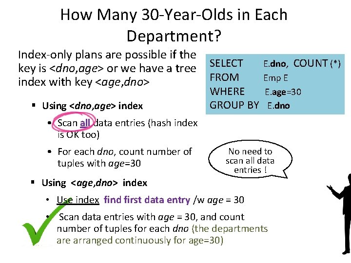
How Many 30 -Year-Olds in Each Department? Index-only plans are possible if the key is <dno, age> or we have a tree SELECT E. dno, COUNT (*) FROM Emp E index with key <age, dno> § Using <dno, age> index WHERE E. age=30 GROUP BY E. dno • Scan all data entries (hash index is OK too) • For each dno, count number of tuples with age=30 No need to scan all data entries ! § Using <age, dno> index • Use index find first data entry /w age = 30 • Scan data entries with age = 30, and count number of tuples for each dno (the departments are arranged continuously for age=30)

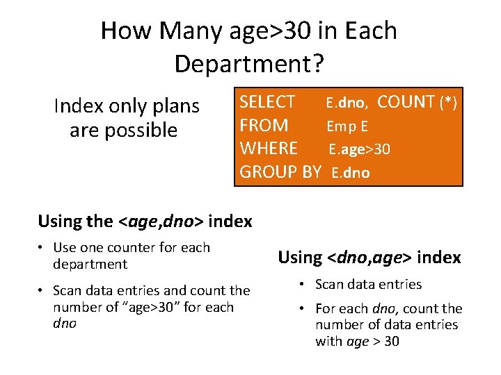
How Many age>30 in Each Department? Index only plans are possible SELECT E. dno, COUNT (*) FROM Emp E WHERE E. age>30 GROUP BY E. dno Using the <age, dno> index • Use one counter for each department • Scan data entries and count the number of “age>30” for each dno Using <dno, age> index • Scan data entries • For each dno, count the number of data entries with age > 30

Summary • Many alternative file organizations exist, each appropriate in some situation. • If selection queries are frequent, sorting the file or building an index is important. – – Hash-based indexes only good for equality search. Sorted files and tree-based indexes best for range search; also good for equality search. (Files rarely kept sorted in practice; B+ tree index is better. ) • Index is: 1) a collection of data entries (<key, rid> pairs or <key, ridlist> pairs), plus 2) a way to quickly find entries (using hashing or a search tree) with given key values.

Summary (Contd. ) • Data entries can be (1) actual data records, (2) <key, rid> pairs, or (3) <key, rid-list> pairs. – Choice orthogonal to indexing technique used to locate data entries with a given key value. • Can have several indexes on a given file of data records, each with a different search key. • Indexes can be classified as clustered vs. unclustered. Differences have important consequences for utility/performance.

Summary (Contd. ) • Understanding the nature of the workload for the application, and the performance goals, is essential to developing a good design. – What are the important queries and updates? What attributes/relations are involved? • Indexes must be chosen to speed up important queries (and perhaps some updates!). – – – Index maintenance overhead on updates to key fields. Choose indexes that can help many queries, if possible. Build indexes to support index-only strategies. Clustering is an important decision; only one index on a given relation can be clustered! Order of fields in composite index key can be important.