Chapter 8 Short Run Costs and Output Decisions

Chapter 8 – Short Run Costs and Output Decisions • Firms need to determine how much Output (Q) to produce to ensure they are Maximizing their Profits. • A firm’s Profit is equal to their Total Revenue (TR) minus their Total Cost (TC). • = TR - TC. 1

Short Run • Once they decide how much Output to produce, they need to decide how much Labor and Capital to use to produce that chosen Q. • Labor and Capital are inputs and the firm has to pay for them. • Therefore, the amount of Labor and Capital the firm uses will affect their Cost of Production. 2

Short Run cont. • The firm’s Cost of Production will behave differently in the Short Run than the Long Run. • This is because in the Short Run, Capital is fixed and only Labor can change. 3

Short Run cont. • Therefore, in the Short Run, a firm’s costs are dominated by the concept of Diminishing Marginal Returns (DMR). • DMR - as labor inputs are successively increased, output is increasing at a decreasing rate. • Since Capital is fixed, the only way for a firm to increase Output is to increase Labor. 4

Cost Curves • Total Costs = Fixed Costs (FC) + Variable Costs (VC). • Fixed Costs - costs that do not depend on the firm’s output. • The firm incurs these costs even if it produces nothing. 5

Fixed Cost cont. • Example: Dominos Pizza • Fixed Costs: tables, chairs, cash register, ovens, equipment, rent. 6

Fixed Cost Curve • Since Fixed Cost do not change with Output, the curve is horizontal. 7

Variable Costs • Variable Costs change when the amount the firm produces (Q) changes. • Example: Dominos Pizza • Variable Cost: Labor, Cheese, Sauce, Dough 8

Variable Cost Curve • As Q increases, the VC will increase as well. 9

Total Costs • Total Costs are the sum of FC and VC. • Total Costs = Fixed Cost + Variable Costs • Since Variable Costs are increasing with Q, Total Costs also increase with Q. • The Total Cost Curve will take on the same shape as the Variable Cost Curve but will lie above Variable Costs. 10

Total Cost Curve • Total Cost lies above the Variable Cost Curve because Total Costs also includes Fixed Costs. 11

TC, VC, and FC Graph 12

Average Fixed Costs (AFC) • AFC = FC ÷ Q. • This is a per unit measure of Fixed Costs. • As the firm’s Output increases, Average Fixed Cost decreases. 13

Average Fixed Cost Curve 14

Average Variable Costs (AVC) • AVC = VC ÷ Q. • This shows Variable Cost per unit of Output. • Average Variable Cost looks like a wide U (upside down rainbow!) 15

AVC Curve 16

Average Total Costs (ATC) • Average Total Cost = TC ÷ Q. • This is a per unit measure of Total Cost. • We can also calculate ATC summing AFC and AVC: • Average Total Cost = AFC + AVC. 17

ATC Curve cont. • The Average Total Cost Curve will have the same shape as the Average Variable Cost Curve. (Upside down rainbow!) • However, the ATC Curve will lie above the AVC Curve. • The ATC Curve lies above AVC because ATC also includes AFC. 18

AVC and ATC Curves 19

Marginal Costs (MC) • Marginal Cost = TC ÷ Q. • This represents the change in Total Cost from producing one more unit of Output. • MC looks like a wide J (candy cane!) 20

Marginal Cost Curve • MC will decline at first and then it begins to rise. 21

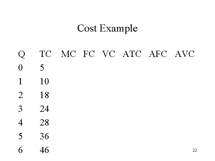
Cost Example Q 0 1 2 3 4 5 6 TC MC FC VC ATC AFC AVC 5 10 18 24 28 36 22 46

Cost Example cont. • From our example, we can graph, TC, VC, FC, ATC, AVC, AFC, and MC. • We will always graph the Total Cost Curves on one graph, and the Average and Marginal Cost Curves on a separate graph. 23

TC, FC, and VC Graph 24

ATC, AVC, and MC Graph 25

Rules for Marginal/Average Cost Curves • 1) The MC curve cuts through the ATC and AVC curves at their minimum points. • 2) The minimum point on AVC is below and to the left of the minimum point on ATC.

Rules cont. • 3) The MC curve pulls the ATC curve. • a) When MC > ATC, ATC is rising. • b) When MC < ATC, ATC is falling. • c) When MC = ATC, ATC is constant. 27

Average and Marginal Cost Curve Graph 28

Cost Curves: Important Points • 1) The slope of the Marginal Cost Curve is due to the Law of Diminishing Marginal Returns to Labor: • The Marginal Cost Curve is a flipped image of the Marginal Product of Labor Curve.

Points cont. • When Labor is first hired, MPL is rising and MC is falling. • This is because there are high returns when the firm first begins to hire Labor. • Since returns are so high, it implies cost per worker are falling. 30

MC and MPL Curves

Important Points cont. • As the firm hires more and more Labor, Marginal Product begins to fall because each additional worker is producing less and less output. • Since each worker is producing less and less output, it implies cost per worker (MC) is rising. • Therefore, the slope of the MC curve is due to the presence of Diminishing Marginal Returns to Labor.

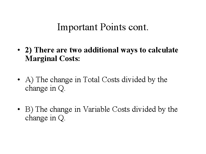
Important Points cont. • 2) There are two additional ways to calculate Marginal Costs: • A) The change in Total Costs divided by the change in Q. • B) The change in Variable Costs divided by the change in Q.

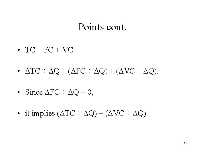
Points cont. • TC = FC + VC. • ΔTC ÷ ΔQ = (ΔFC ÷ ΔQ) + (ΔVC ÷ ΔQ). • Since ΔFC ÷ ΔQ = 0, • it implies (ΔTC ÷ ΔQ) = (ΔVC ÷ ΔQ). 34

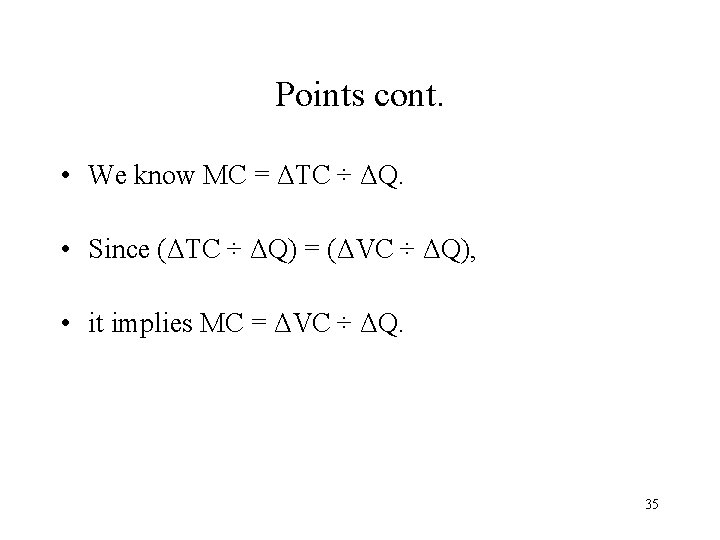
Points cont. • We know MC = ΔTC ÷ ΔQ. • Since (ΔTC ÷ ΔQ) = (ΔVC ÷ ΔQ), • it implies MC = ΔVC ÷ ΔQ. 35

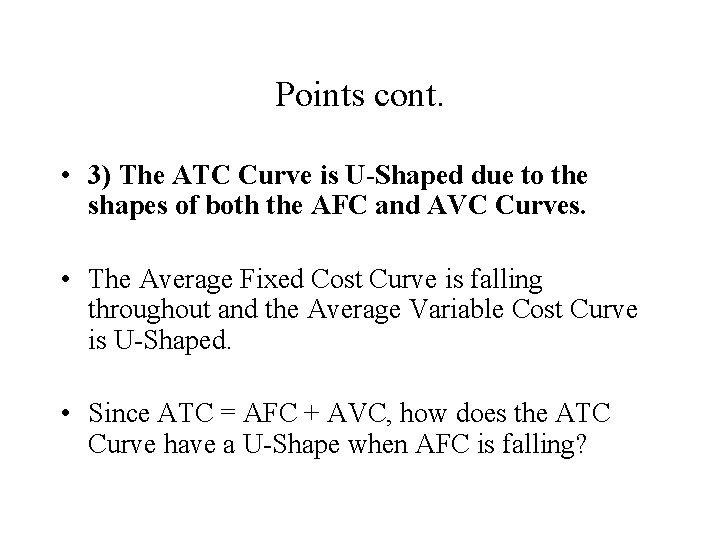
Points cont. • 3) The ATC Curve is U-Shaped due to the shapes of both the AFC and AVC Curves. • The Average Fixed Cost Curve is falling throughout and the Average Variable Cost Curve is U-Shaped. • Since ATC = AFC + AVC, how does the ATC Curve have a U-Shape when AFC is falling?

ATC, AFC, and AVC Curves

Important Points cont. • At low levels of Q, Average Fixed Cost is falling and Average Variable Cost is falling. • Therefore, at low levels of Q, Average Total Cost is also falling.

Points cont. • At higher levels of Q, AFC is falling and AVC is rising. • However, AVC is rising by more than AFC is falling. • Therefore, the AVC increase outweighs the AFC decrease, causing the overall effect to result in an increase in ATC. 39