Chapter 8 Reasoning Under Uncertainty Part I Main

Chapter 8 Reasoning Under Uncertainty – Part I Main Textbook: Artificial Intelligence Foundations of Computational Agents, 2 nd Edition, David L. Poole and Alan K Mackworth, Cambridge University Press, 2018. Reference Textbook: Artificial Intelligence: A Guide to Intelligence Systems, Michael Negnevitsky, 3 rd Edition, 2011, Addison Wesley, ISBN 978 -1408225745 Asst. Prof. Dr. Anilkumar K. G 1

Introduction • Agents in real environments are inevitably forced to make decisions based on incomplete information. • Even when an agent senses the world to find out more information, it rarely finds out the exact state of the world – For example, a doctor does not know exactly what is going on inside a patient, a teacher does not know exactly what a student understands, etc. • This chapter considers reasoning with uncertainty that arises whenever an agent is not omniscient – This chapter describes how probability can be used to represent the world by making appropriate independence assumptions, and shows how to reason with such representations. Asst. Prof. Dr. Anilkumar K. G 2

Probability • Reasoning with uncertainty has been studied in the fields of probability theory and decision theory. • When an agent makes decisions and is uncertain about the outcomes of its actions, it is gambling on the outcomes. – We have learnt that probability as theory of tossing coins and rolling dice. • In general, probability is a calculus for belief designed for making decisions – Probability theory is the study of how knowledge affects belief is measured in terms of a number between 0 and 1 • The probability of belief α is 0 means that α is believed to be definitely false, and the probability of α is 1 means that α is believed to be definitely true. Asst. Prof. Dr. Anilkumar K. G 3

Probability • Probability is a measure of belief and the belief need to be updated when a new evidence is observed. • If an agent’s probability of belief α is greater than 0 and less than 1, this does not mean that α is true to some degree – but rather that the agent is ignorant of whether α is true or false. • The view of probability as a measure of belief is known as Bayesian probability or subjective probability. – Uncertainty in the world is epistemological – pertaining to an agent’s beliefs of the world, rather than ontological – how the world is. Asst. Prof. Dr. Anilkumar K. G 4

Semantics of Probability • Probability theory is built on the foundation of worlds and variables – Variables could be described in terms of worlds; a variable is a function from worlds into the domain of the variable. • Variables will be written starting with an uppercase letter. • Each variable has a domain which is the set of values that the variable can take – A Boolean variable is a variable with domain {true, false}. – A discrete variable has a domain that is a finite set. For example, a world could consist of the symptoms, diseases and test results. • We might be able to answer questions about the probability that a patient with a particular combination of symptoms may come into the hospital again in the nearby future. Asst. Prof. Dr. Anilkumar K. G 5

Semantics of Probability • We first define a probability over finite sets of worlds with finitely many variables and use this to define the probability of propositions. • A probability measure is a function P from worlds into the nonnegative real numbers such that, – where Ω is the set of all possible worlds. – The use of 1 as the probability of the set of all of the worlds is just by convention. • The probability of proposition α, written P(α), is the sum of the probabilities of possible worlds in which α is true. Asst. Prof. Dr. Anilkumar K. G 6

Semantics of Probability Asst. Prof. Dr. Anilkumar K. G 7

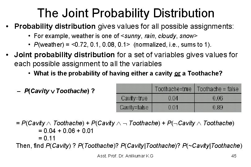
Semantics of Probability • If X is a random variable, a probability distribution, P(X), over X is a function from the domain of X into the real numbers such that, given a value x ∈ domain(X), P(x) is the probability of the proposition X = x. • A probability distribution over a set of variables is a function from the values of those variables into a probability – For example, P(X, Y) is a probability distribution over X and Y such that P(X=x, Y=y), where x ∈ domain(X) and y ∈ domain(Y), has the value P(X=x ∧ Y=y), where X=x ∧ Y=y is a proposition and P is the function on propositions defined above. • If (X 1. . . Xn) are random variables, probability distribution over all worlds, P(X 1, . . . , Xn) is called the joint probability distribution. Asst. Prof. Dr. Anilkumar K. G 8

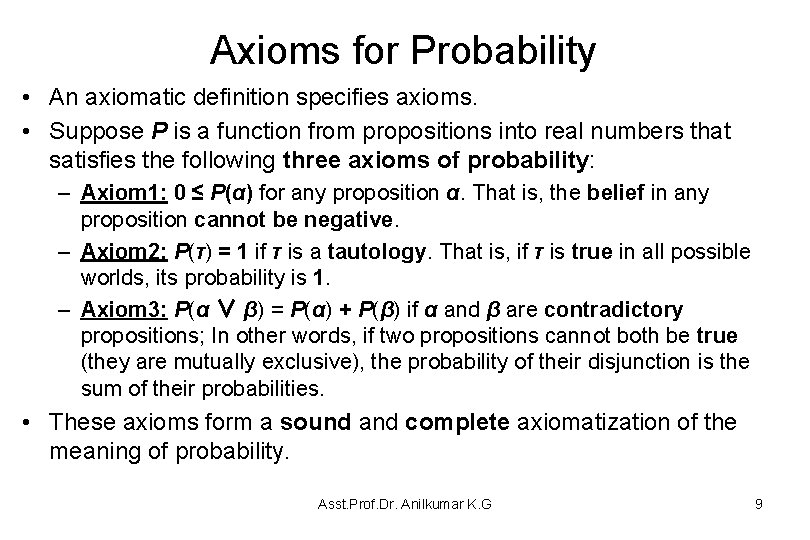
Axioms for Probability • An axiomatic definition specifies axioms. • Suppose P is a function from propositions into real numbers that satisfies the following three axioms of probability: – Axiom 1: 0 ≤ P(α) for any proposition α. That is, the belief in any proposition cannot be negative. – Axiom 2: P(τ) = 1 if τ is a tautology. That is, if τ is true in all possible worlds, its probability is 1. – Axiom 3: P(α ∨ β) = P(α) + P(β) if α and β are contradictory propositions; In other words, if two propositions cannot both be true (they are mutually exclusive), the probability of their disjunction is the sum of their probabilities. • These axioms form a sound and complete axiomatization of the meaning of probability. Asst. Prof. Dr. Anilkumar K. G 9

Axioms for Probability • Proposition 8. 1: If there a finite number of discrete random variables, Axioms 1, 2, and 3 are sound and complete with respect to the semantics. • Proposition 8. 2: The following hold for all propositions α and β – (a) Negation of a proposition: P(￢α) = 1 − P(α). – (b) If α ↔ β, then P(α) = P(β). That is, logically equivalent propositions have the same probability. – (c) Reasoning by cases: P(α) = P(α ∧ β) + P(α ∧ ￢β). – (d) If V is a random variable with domain D, then, for all propositions α, – (e) Disjunction for non-exclusive propositions: P(α ∨ β) = P(α) + P(β) −P(α ∧ β). Asst. Prof. Dr. Anilkumar K. G 10

Axioms for Probability • Proof. (a): The propositions α ∨ ￢α and ￢(α ∧ ￢α) are tautologies. Therefore, 1 = P(α ∨ ￢α) = P(α) +P(￢α). Rearranging gives the desired result. • Proof. (b): If α ↔ β, then α ∨ ￢β is a tautology, so P(α ∨ ￢β) = 1. α and ￢β are contradictory statements, so Axiom 3 gives P(α ∨ ￢β) = P(α) + P(￢β). Using part (a), P(￢β) = 1 − P(β). Thus, P(α) + 1 − P(β) = 1, and so P(α) = P(β). • Proof. (c): The proposition α ↔ ((α ∧ β) ∨ (α ∧ ￢β)) and ￢((α ∧ β) ∧ (α ∧ ￢β)) are tautologies. Thus, P(α) = P((α ∧ β) ∨ (α ∧ ￢β)) = P(α ∧ β) +P(α ∧ ￢β). • Proof. (d): The proof is analogous to the proof of proposition (c). • Proof. (e): (α ∨ β)↔ ((α ∧ ￢β) ∨ β) is a tautology. Thus, P(α ∨ β) = P((α ∧ ￢β) ∨ β) = P(α ∧ ￢β) +P(β). Proposition (c) shows P(α ∧ ￢β) = P(α)− P(α ∧ β). Thus, P(α ∨ β) = P(α) + P(β) −P(α ∧ β). Asst. Prof. Dr. Anilkumar K. G 11

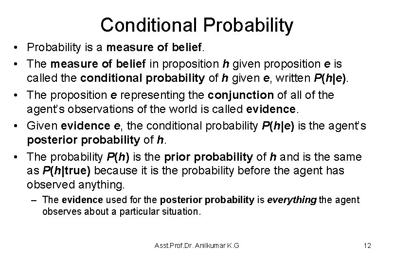
Conditional Probability • Probability is a measure of belief. • The measure of belief in proposition h given proposition e is called the conditional probability of h given e, written P(h|e). • The proposition e representing the conjunction of all of the agent’s observations of the world is called evidence. • Given evidence e, the conditional probability P(h|e) is the agent’s posterior probability of h. • The probability P(h) is the prior probability of h and is the same as P(h|true) because it is the probability before the agent has observed anything. – The evidence used for the posterior probability is everything the agent observes about a particular situation. Asst. Prof. Dr. Anilkumar K. G 12

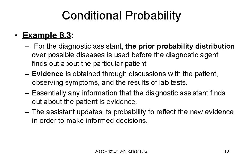
Conditional Probability • Example 8. 3: – For the diagnostic assistant, the prior probability distribution over possible diseases is used before the diagnostic agent finds out about the particular patient. – Evidence is obtained through discussions with the patient, observing symptoms, and the results of lab tests. – Essentially any information that the diagnostic assistant finds out about the patient is evidence. – The assistant updates its probability to reflect the new evidence in order to make informed decisions. Asst. Prof. Dr. Anilkumar K. G 13

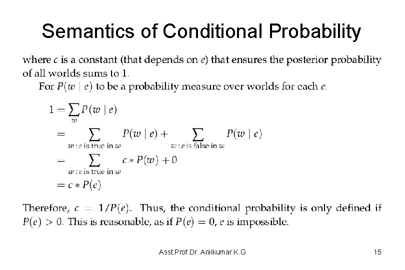
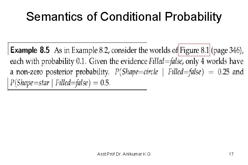
Semantics of Conditional Probability • Evidence e, where e is a proposition, will rule out all possible worlds that are incompatible with e. – Like the definition of logical consequence, the given proposition e selects the possible worlds in which e is true. – As in the definition of probability, we first define the conditional probability over worlds, and then use this to define a probability over propositions. • Evidence e induces a new probability P(w|e) of world w given e. Any world where e is false has conditional probability 0, and the remaining worlds are normalized so that the probabilities of the worlds sum to 1: c x P(w) if e is true in world w P(w|e) = 0 if e is false in world w – where c is a constant (depends on e) that ensures the posterior probability of all worlds sums to 1. Asst. Prof. Dr. Anilkumar K. G 14

Semantics of Conditional Probability Asst. Prof. Dr. Anilkumar K. G 15

Semantics of Conditional Probability Asst. Prof. Dr. Anilkumar K. G 16

Semantics of Conditional Probability Asst. Prof. Dr. Anilkumar K. G 17

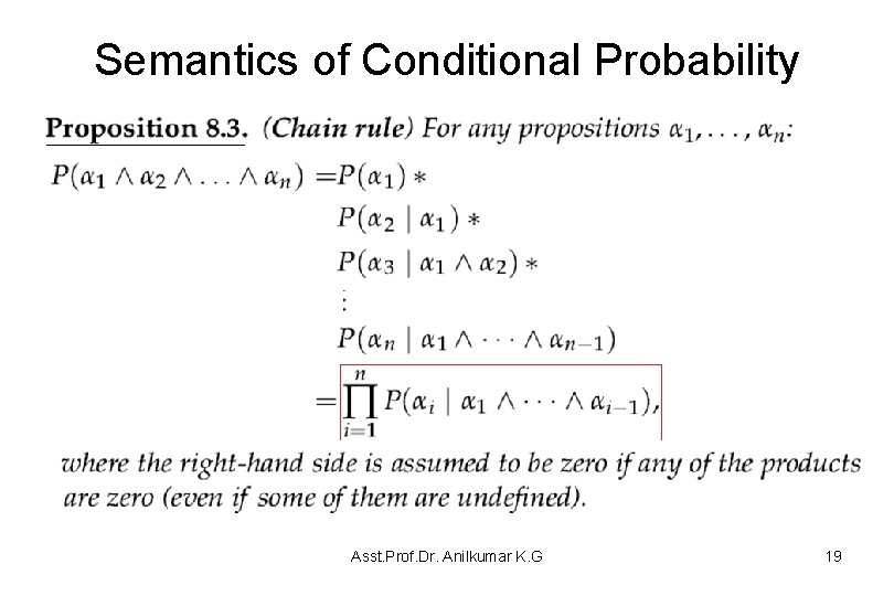
Semantics of Conditional Probability • A conditional probability distribution, written P(X|Y) where X and Y are variables or sets of variables, is a function of the variables: given a value x ∈ domain(X) for X and a value y ∈ domain(Y) for Y, it gives the value P(X = x|Y = y), where the latter is the conditional probability of the propositions. • The definition of conditional probability allows the decomposition of a conjunction into a product of conditional probabilities: Asst. Prof. Dr. Anilkumar K. G 18

Semantics of Conditional Probability Asst. Prof. Dr. Anilkumar K. G 19

Axioms of probability: Summary 1. 0 £ P(A) £ 1 ; for every A S (S is the given finite sample space) 2. Boundary: P( ) = 0 and P(S) = 1 3. Monotonic: if A B S, then p(A) p(B) 4. Inclusion–exclusion: If A and B are mutually inclusive, P(A / B) = P(A)+P(B) P(A / B) If A and B are mutually exclusive, then P(A / B) = P(A) + P(B) 5. 6. 7. Intersection: P(A / B) = P(A)* P(B|A), where A and B are true Negation: P(~A) = 1 P(A), this is a generalization of the fact that A is true if and only if ~A is false and vice versa Equivalence: If A B, then P(A) = P(B) (Assume A and B are two propositions) Asst. Prof. Dr. Anilkumar K. G 20

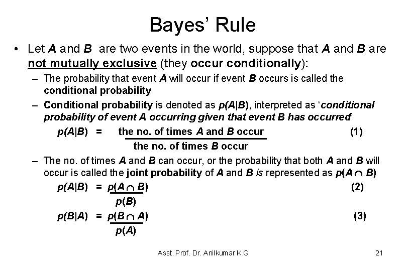
Bayes’ Rule • Let A and B are two events in the world, suppose that A and B are not mutually exclusive (they occur conditionally): – The probability that event A will occur if event B occurs is called the conditional probability – Conditional probability is denoted as p(A|B), interpreted as ‘conditional probability of event A occurring given that event B has occurred’ p(A|B) = the no. of times A and B occur (1) the no. of times B occur – The no. of times A and B can occur, or the probability that both A and B will occur is called the joint probability of A and B is represented as p(A B) p(A|B) = p(A B) (2) p(B|A) = p(B A) (3) p(A) Asst. Prof. Dr. Anilkumar K. G 21

Bayes’ Rule • From (2) and (3) we get p(A B) = p(A|B) x p(B) and p(B A) = p(B|A) x p(A) Joint probability is commutative, thus p(A B) = p(B A), therefore p(A|B) x p(B) = p(B|A) x p(A) Eq. (5) yields the following equation: p(A|B) = p(B|A) x p(A) p(B) (4) (5) (6) • The Eq. (6) is known as Bayes’ rule Where: – p(A|B) is the conditional probability that event A occurs given that event B has occurred – p(B|A) is the conditional probability of event B occurring given that event A has occurred – p(A) is the prior probability of event A – p(B) is the prior probability of event B • Asst. Prof. Dr. Anilkumar K. G 22

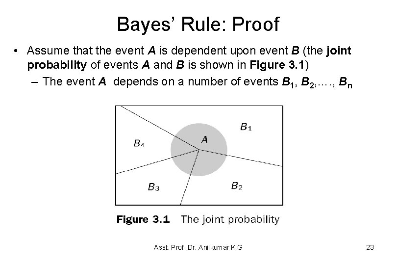
Bayes’ Rule: Proof • Assume that the event A is dependent upon event B (the joint probability of events A and B is shown in Figure 3. 1) – The event A depends on a number of events B 1, B 2, …. , Bn Asst. Prof. Dr. Anilkumar K. G 23

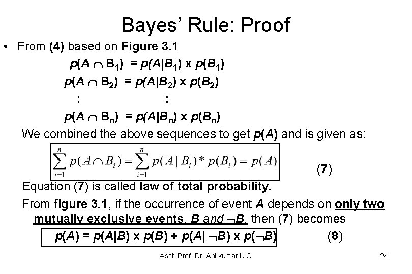
Bayes’ Rule: Proof • From (4) based on Figure 3. 1 p(A B 1) = p(A|B 1) x p(B 1) p(A B 2) = p(A|B 2) x p(B 2) : : p(A Bn) = p(A|Bn) x p(Bn) We combined the above sequences to get p(A) and is given as: (7) Equation (7) is called law of total probability. From figure 3. 1, if the occurrence of event A depends on only two mutually exclusive events, B and B, then (7) becomes p(A) = p(A|B) x p(B) + p(A| B) x p( B) (8) Asst. Prof. Dr. Anilkumar K. G 24

Bayes’ Rule: Proof Similarly, if the occurrence of B depends on events, A and A, then p(B) = p(B|A) x p(A) + p(B| A) x p( A) (9) Substitute (9) into Baye’s rule (6) to yield p(A|B) = p(B|A) x p(A) (10) p(B|A) x p(A) + p(B| A) x p( A) • Eq. (10) provides the background for the application of probability theory to mange uncertainty. Asst. Prof. Dr. Anilkumar K. G 25

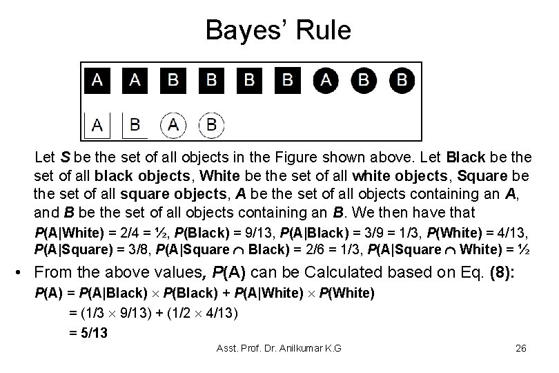
Bayes’ Rule Let S be the set of all objects in the Figure shown above. Let Black be the set of all black objects, White be the set of all white objects, Square be the set of all square objects, A be the set of all objects containing an A, and B be the set of all objects containing an B. We then have that P(A|White) = 2/4 = ½, P(Black) = 9/13, P(A|Black) = 3/9 = 1/3, P(White) = 4/13, P(A|Square) = 3/8, P(A|Square Black) = 2/6 = 1/3, P(A|Square White) = ½ • From the above values, P(A) can be Calculated based on Eq. (8): P(A) = P(A|Black) P(Black) + P(A|White) P(White) = (1/3 9/13) + (1/2 4/13) = 5/13 Asst. Prof. Dr. Anilkumar K. G 26

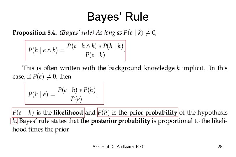
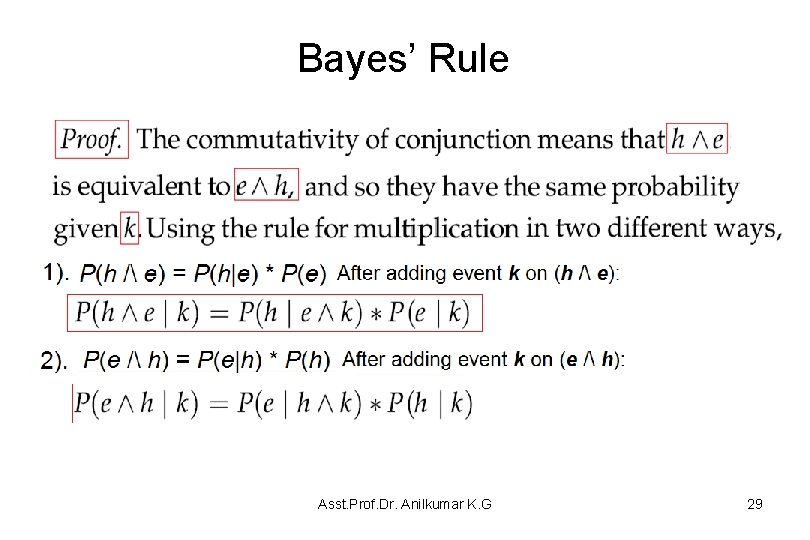
Bayes’ Rule • An agent using probability to update its belief when it observes a new evidence – The new evidence is conjoined to the old evidence to form a complete evidence. • Bayes’ rule specifies how an agent should update its belief based on a new evidence: – Suppose an agent has a current belief in proposition h (called hypothesis) based on evidence k, can be given by P(h|k), and can subsequently observes with a new evidence e: P(h|(e ∧ k)). – Bayes’ rule tells us how to update the agent’s belief in hypothesis h as new evidence arrives. Asst. Prof. Dr. Anilkumar K. G 27

Bayes’ Rule Asst. Prof. Dr. Anilkumar K. G 28

Bayes’ Rule Asst. Prof. Dr. Anilkumar K. G 29

Bayes’ Rule Asst. Prof. Dr. Anilkumar K. G 30

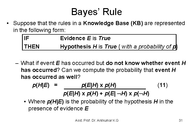
Bayes’ Rule • Suppose that the rules in a Knowledge Base (KB) are represented in the following form: IF Evidence E is True THEN Hypothesis H is True { with a probability of p} – What if event E has occurred but do not know whether event H has occurred? Can we compute the probability that event H has occurred as well? p(H|E) = p(E|H) x p(H) (11) p(E|H) x p(H) + p(E| H) x p( H) • Where p(H|E) is the probability of the hypothesis H in the presence of evidence E Asst. Prof. Dr. Anilkumar K. G 31

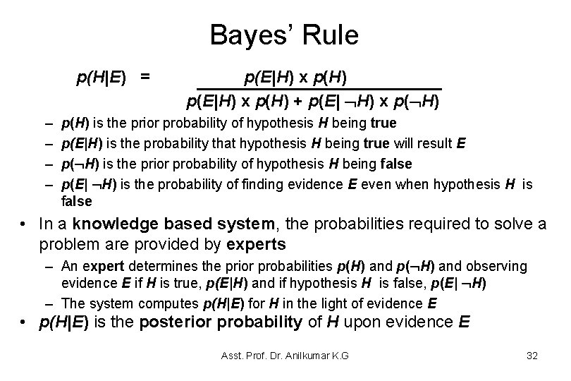
Bayes’ Rule p(H|E) = – – p(E|H) x p(H) + p(E| H) x p( H) p(H) is the prior probability of hypothesis H being true p(E|H) is the probability that hypothesis H being true will result E p( H) is the prior probability of hypothesis H being false p(E| H) is the probability of finding evidence E even when hypothesis H is false • In a knowledge based system, the probabilities required to solve a problem are provided by experts – An expert determines the prior probabilities p(H) and p( H) and observing evidence E if H is true, p(E|H) and if hypothesis H is false, p(E| H) – The system computes p(H|E) for H in the light of evidence E • p(H|E) is the posterior probability of H upon evidence E Asst. Prof. Dr. Anilkumar K. G 32

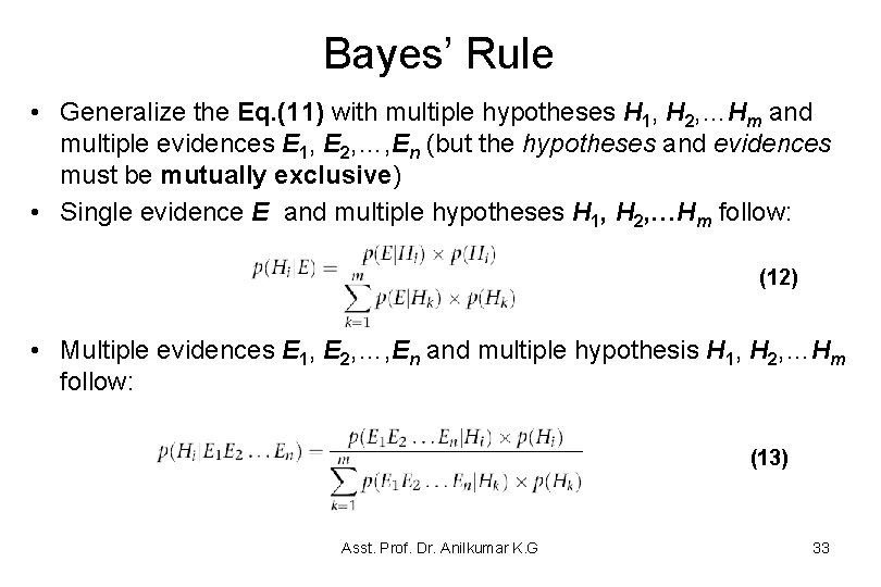
Bayes’ Rule • Generalize the Eq. (11) with multiple hypotheses H 1, H 2, …Hm and multiple evidences E 1, E 2, …, En (but the hypotheses and evidences must be mutually exclusive) • Single evidence E and multiple hypotheses H 1, H 2, …Hm follow: (12) • Multiple evidences E 1, E 2, …, En and multiple hypothesis H 1, H 2, …Hm follow: (13) Asst. Prof. Dr. Anilkumar K. G 33

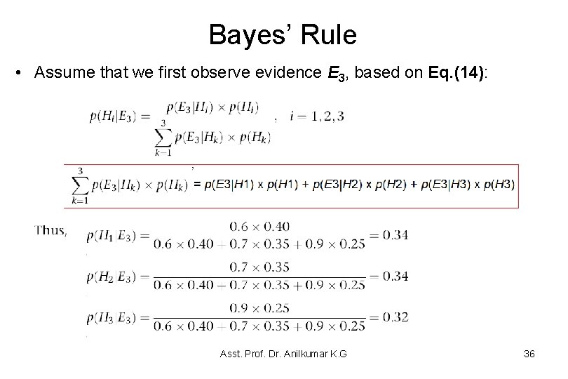
Bayes’ Rule • An application of Eq. (13) requires to obtain the conditional probabilities of all possible combinations of evidences for all hypothesis; (14) • How does an ES compute all posterior probabilities and finally rank potentially true hypothesis? – Suppose an ES, given three conditionally independent evidences E 1, E 2, and E 3 creates three mutually exclusive hypothesis H 1, H 2, and H 3 and provides prior probabilities for these hypothesis- p(H 1), p(H 2) and p(H 3) respectively • Table 3. 2 illustrates the prior and conditional probabilities provided by the expert Asst. Prof. Dr. Anilkumar K. G 34

Bayes’ Rule Asst. Prof. Dr. Anilkumar K. G 35

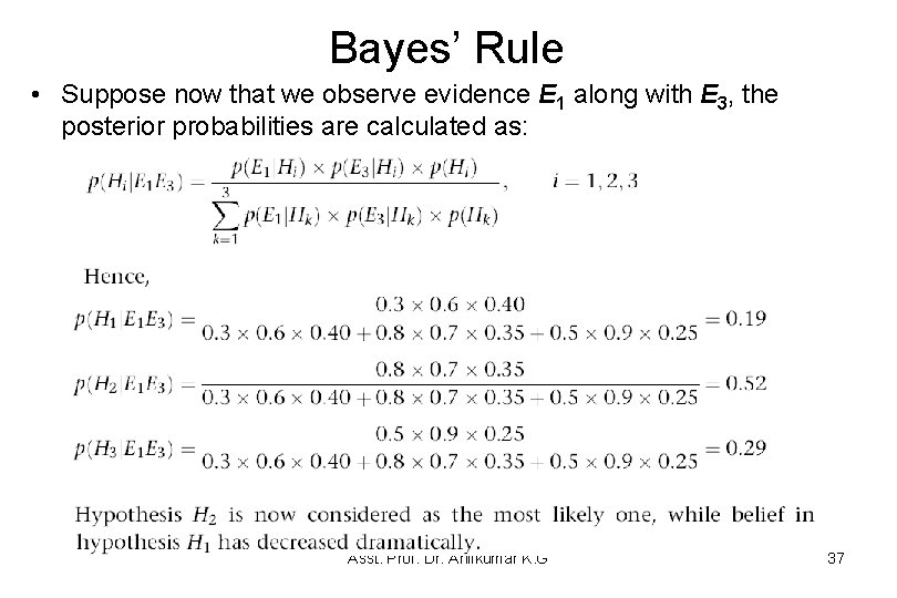
Bayes’ Rule • Assume that we first observe evidence E 3, based on Eq. (14): Asst. Prof. Dr. Anilkumar K. G 36

Bayes’ Rule • Suppose now that we observe evidence E 1 along with E 3, the posterior probabilities are calculated as: Asst. Prof. Dr. Anilkumar K. G 37

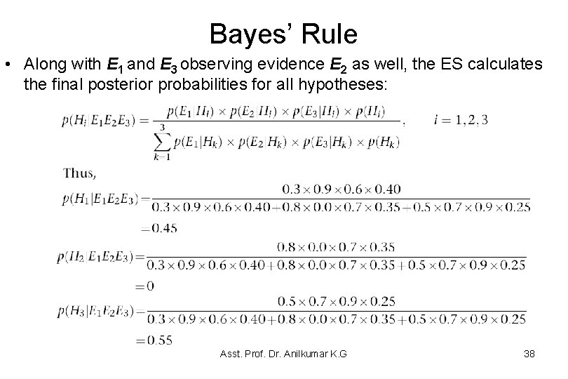
Bayes’ Rule • Along with E 1 and E 3 observing evidence E 2 as well, the ES calculates the final posterior probabilities for all hypotheses: Asst. Prof. Dr. Anilkumar K. G 38

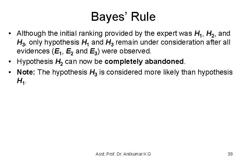
Bayes’ Rule • Although the initial ranking provided by the expert was H 1, H 2, and H 3, only hypothesis H 1 and H 3 remain under consideration after all evidences (E 1, E 2 and E 3) were observed. • Hypothesis H 2 can now be completely abandoned. • Note: The hypothesis H 3 is considered more likely than hypothesis H 1. Asst. Prof. Dr. Anilkumar K. G 39

Exercises 1. Prove p(A B) = p(A) + p(B) p(A B) {where A and B are not mutually exclusive events}. 2. Prove that p(A B) = p(~A) + p(B) – p(~A B) { where A and B are not mutually exclusive events}. 3. Show, P(A| B A) = 1 4. Consider an incandescent bulb manufacturing unit. Here machines M 1, M 2 and M 3 make 20%, 30% and 50% of the total bulbs. Of their output, let's assume that 2%, 3% and 5% are defective. A bulb is drawn at random and is found defective. What is the probability that the bulb is made by machine M 1 or M 2 or M 3. Asst. Prof. Dr. Anilkumar K. G 40

Asst. Prof. Dr. Anilkumar K. G 41

Asst. Prof. Dr. Anilkumar K. G 42

Asst. Prof. Dr. Anilkumar K. G 43

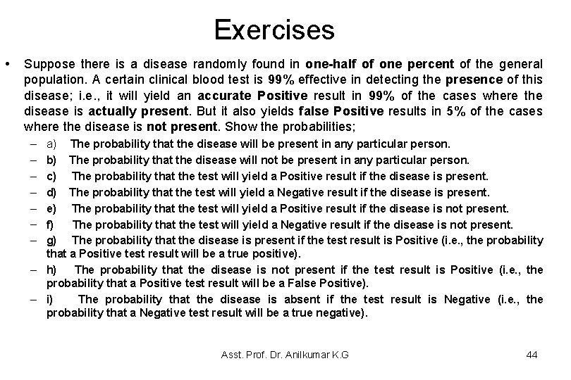
Exercises • Suppose there is a disease randomly found in one-half of one percent of the general population. A certain clinical blood test is 99% effective in detecting the presence of this disease; i. e. , it will yield an accurate Positive result in 99% of the cases where the disease is actually present. But it also yields false Positive results in 5% of the cases where the disease is not present. Show the probabilities; – – – – a) The probability that the disease will be present in any particular person. b) The probability that the disease will not be present in any particular person. c) The probability that the test will yield a Positive result if the disease is present. d) The probability that the test will yield a Negative result if the disease is present. e) The probability that the test will yield a Positive result if the disease is not present. f) The probability that the test will yield a Negative result if the disease is not present. g) The probability that the disease is present if the test result is Positive (i. e. , the probability that a Positive test result will be a true positive). – h) The probability that the disease is not present if the test result is Positive (i. e. , the probability that a Positive test result will be a False Positive). – i) The probability that the disease is absent if the test result is Negative (i. e. , the probability that a Negative test result will be a true negative). Asst. Prof. Dr. Anilkumar K. G 44

The Joint Probability Distribution • Probability distribution gives values for all possible assignments: • For example, weather is one of <sunny, rain, cloudy, snow> • P(weather) = <0. 72, 0. 1, 0. 08, 0. 1> (normalized, i. e. , sums to 1). • Joint probability distribution for a set of variables gives values for each possible assignment to all the variables • What is the probability of having either a cavity or a Toothache? – P(Cavity Ú Toothache) ? = P(Cavity Toothache) + P(Cavity Toothache) + P( Cavity Toothache) = 0. 04 + 0. 06 + 0. 01 = 0. 11 Then, find P(Cavity) ? P(Toothache)? P(Cavity|Toothache)? P(~Cavity|Toothache) Asst. Prof. Dr. Anilkumar K. G 45

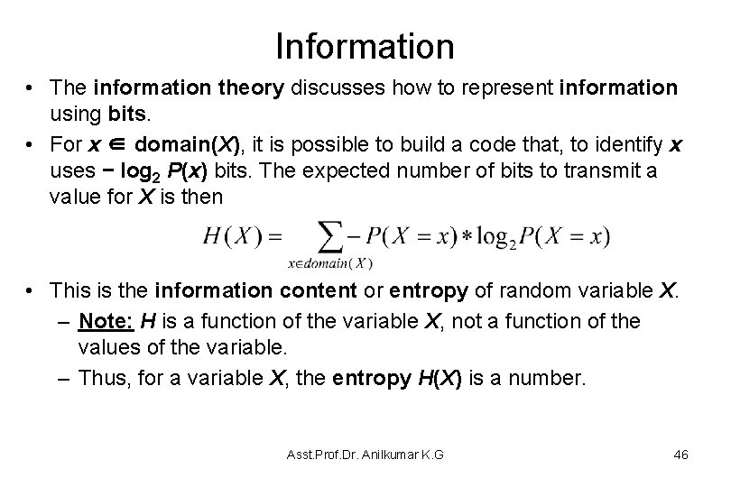
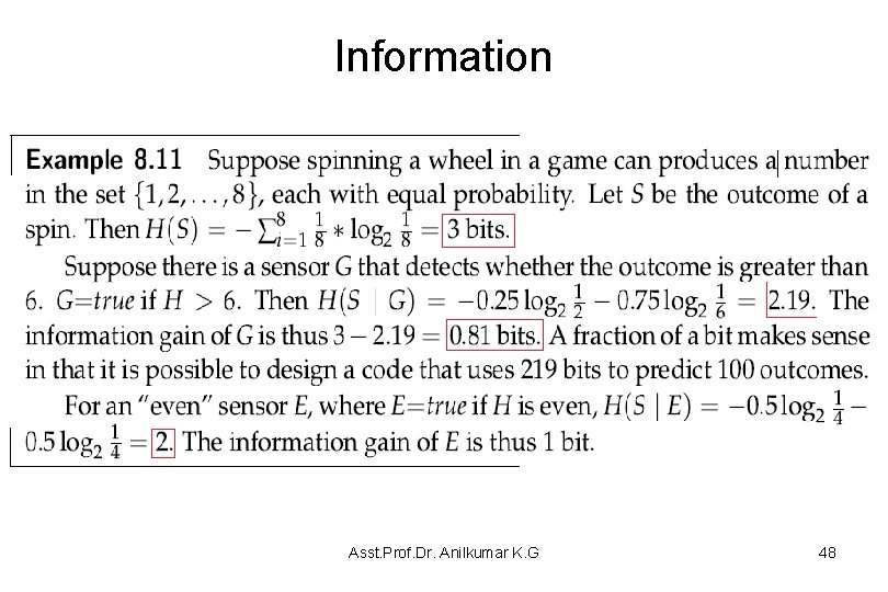
Information • The information theory discusses how to represent information using bits. • For x ∈ domain(X), it is possible to build a code that, to identify x uses − log 2 P(x) bits. The expected number of bits to transmit a value for X is then • This is the information content or entropy of random variable X. – Note: H is a function of the variable X, not a function of the values of the variable. – Thus, for a variable X, the entropy H(X) is a number. Asst. Prof. Dr. Anilkumar K. G 46

Information Asst. Prof. Dr. Anilkumar K. G 47

Information Asst. Prof. Dr. Anilkumar K. G 48

Information • The notion of information is used for a number of tasks: – In diagnosis, an agent could choose a test that provides the most information. – In decision tree learning, information theory provides a useful criterion for choosing which property to split on: split on the property that provides the greatest information gain. – In Bayesian learning, information theory provides a basis for deciding which is the best model given some data. Asst. Prof. Dr. Anilkumar K. G 49

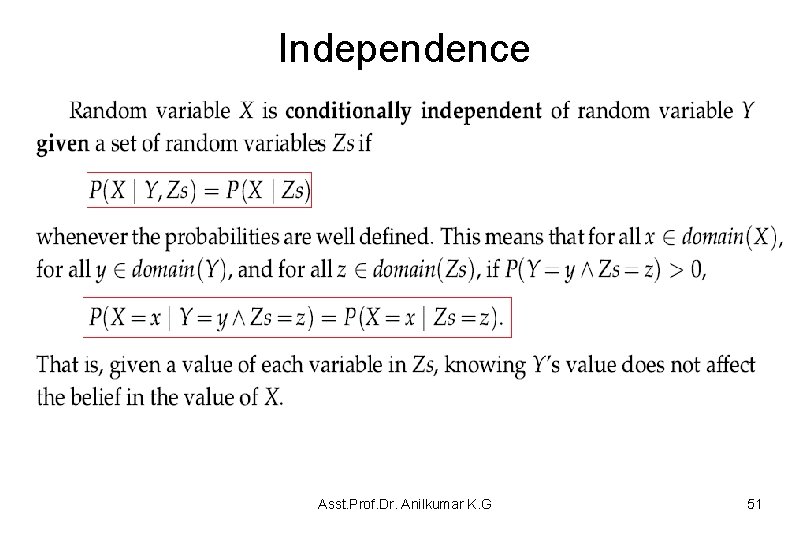
Independence • The axioms of probability are very weak and provide few constraints on allowable conditional probabilities. • A useful way to limit the amount of information required is to assume that each variable only directly depends on a few other variables. • This uses assumptions of conditional independence. • As long as the value of P(h|e) is not 0 or 1, the value of P(h|e) does not constrain the value of P(h|f∧e). • This latter probability could have any value in the range [0, 1]. It is 1 when f implies h, and it is 0 if f implies ￢h. • Certain knowledge in P(h|e) = P(h|f∧e) specifies f is irrelevant (f is 1) to the probability of h given that e is observed. Asst. Prof. Dr. Anilkumar K. G 50

Independence Asst. Prof. Dr. Anilkumar K. G 51

Belief Networks • A belief network is a directed model of conditional dependence among a set of random variables. • The conditional independence in a belief network takes in an ordering of the variables, and results in a directed graph. • To define a belief network on a set of random variables, {X 1, . . . , Xn}, first select a total ordering of the variables, say, X 1, . . . , Xn – The chain rule shows (see proposition 8. 3) how to decompose a conjunction into conditional probabilities: – Define the parents of random variable Xi , written parents(Xi), to be a minimal set of predecessors of Xi in the total ordering such that the other predecessors of Xi are conditionally independent of Xi given parents(Xi). Asst. Prof. Dr. Anilkumar K. G 52

Chain Rule Asst. Prof. Dr. Anilkumar K. G 53

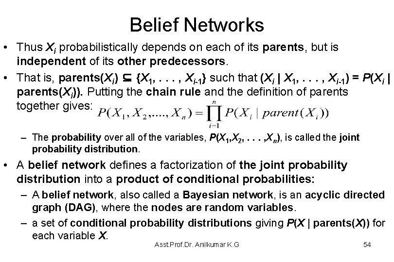
Belief Networks • Thus Xi probabilistically depends on each of its parents, but is independent of its other predecessors. • That is, parents(Xi) ⊆ {X 1, . . . , Xi-1} such that (Xi | X 1, . . . , Xi-1) = P(Xi | parents(Xi)). Putting the chain rule and the definition of parents together gives: – The probability over all of the variables, P(X 1, X 2, . . . , Xn), is called the joint probability distribution. • A belief network defines a factorization of the joint probability distribution into a product of conditional probabilities: – A belief network, also called a Bayesian network, is an acyclic directed graph (DAG), where the nodes are random variables. – a set of conditional probability distributions giving P(X | parents(X)) for each variable X. Asst. Prof. Dr. Anilkumar K. G 54

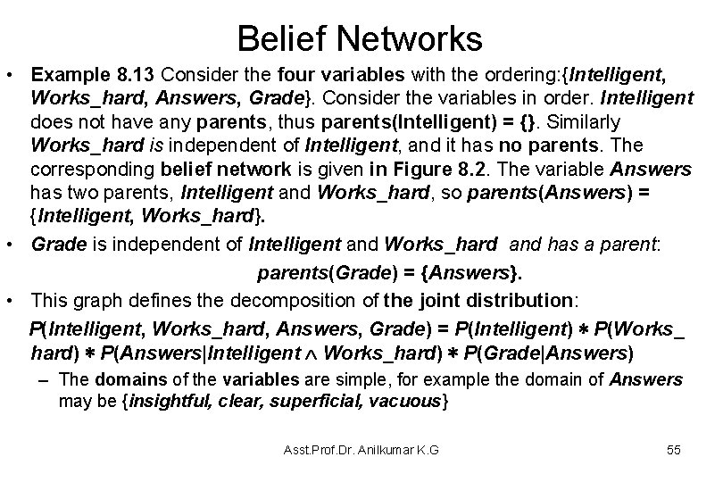
Belief Networks • Example 8. 13 Consider the four variables with the ordering: {Intelligent, Works_hard, Answers, Grade}. Consider the variables in order. Intelligent does not have any parents, thus parents(Intelligent) = {}. Similarly Works_hard is independent of Intelligent, and it has no parents. The corresponding belief network is given in Figure 8. 2. The variable Answers has two parents, Intelligent and Works_hard, so parents(Answers) = {Intelligent, Works_hard}. • Grade is independent of Intelligent and Works_hard and has a parent: parents(Grade) = {Answers}. • This graph defines the decomposition of the joint distribution: P(Intelligent, Works_hard, Answers, Grade) = P(Intelligent) ∗ P(Works_ hard) ∗ P(Answers|Intelligent Works_hard) ∗ P(Grade|Answers) – The domains of the variables are simple, for example the domain of Answers may be {insightful, clear, superficial, vacuous} Asst. Prof. Dr. Anilkumar K. G 55

Belief Networks • A belief network specifies a joint probability distribution from which arbitrary conditional probabilities can be derived. Asst. Prof. Dr. Anilkumar K. G 56

Observations and Queries • Example 8. 14: Before there any observations, the distribution over intelligence is P(Intelligent), which is provided as part of the network. • To determine the distribution over grades, P(Grade), requires inference. • If a grade of A is observed, the posterior distribution of Intelligent is given by: P(Intelligent|Grade=A); intelligent in the presence of grade A • If it was observed that Works_hard is false, the posterior distribution of Intelligent is: P(Intelligent|Grade=A ∧ Works_hard = false). – Although Intelligent and Works_hard are independent as per the given observations, they are dependent given the grade. • This might explain why some people claim they did not work hard to get a good grade; it increases the probability that they are intelligent. Asst. Prof. Dr. Anilkumar K. G 57

Constructing Belief Networks • To represent a domain in a belief network, the designer of a network must consider the following questions: – What are the relevant variables? what the agent may observe in the domain. what information the agent is interested in knowing the posterior probability of. What the other hidden variables or latent variables that will not be observed or queried but make the model simpler. – What values should these variables take? For each variable, the designer should specify what it means to take each value in its domain. – What is the relationship between the variables? This should be expressed by adding arcs in the graph to define the parent relation. – How does the distribution of a variable depend on its parents? This is expressed in terms of the conditional probability distributions. Asst. Prof. Dr. Anilkumar K. G 58

Asst. Prof. Dr. Anilkumar K. G 59

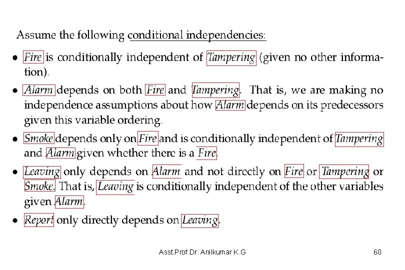
Asst. Prof. Dr. Anilkumar K. G 60

Asst. Prof. Dr. Anilkumar K. G 61

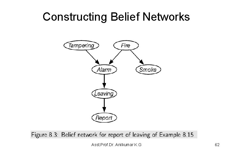
Constructing Belief Networks Asst. Prof. Dr. Anilkumar K. G 62

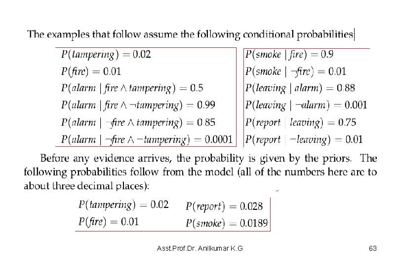
Asst. Prof. Dr. Anilkumar K. G 63

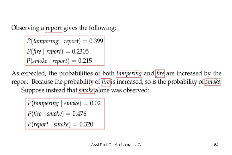
Asst. Prof. Dr. Anilkumar K. G 64

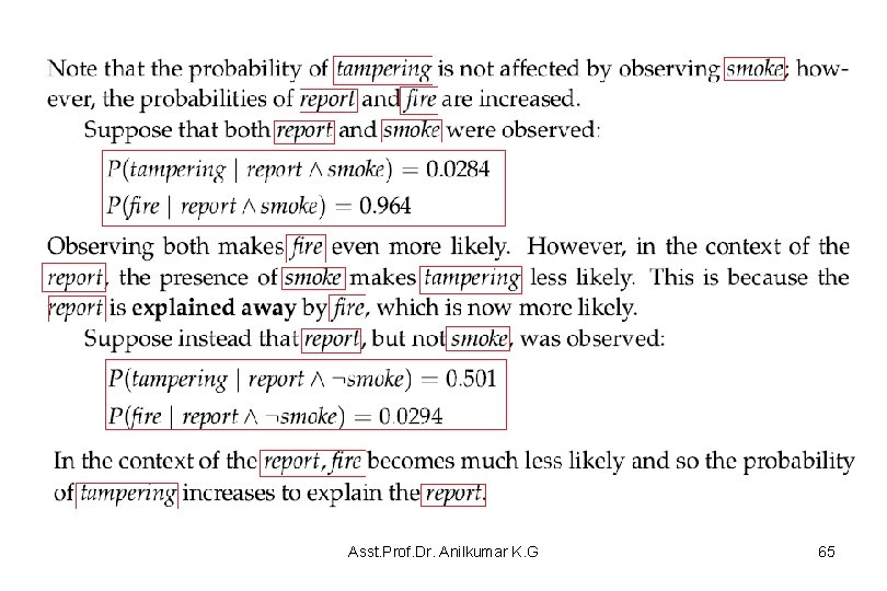
Asst. Prof. Dr. Anilkumar K. G 65

Constructing Belief Networks • Consider the following situation You have a new burglar alarm installed at home. It is fairly reliable at detecting a burglary, but also responds to minor earthquakes. You have two neighbors, John and Marry, who have promised to call you at work when they hear the alarm. John always calls when he hears the alarm, but some times confuses the telephone ringing with the alarm and calls then. Marry on the other hand, likes rather loud music and sometimes misses the alarm. Given evidence of who has or has not called, we would like to estimate the probability of a burglary. • In the case of burglary network, burglary and earthquakes directly effect the probability of the alarm, but John and Marry call depends only on the alarm, that is the network represents that they do not perceive any burglaries directly, and they do not feel the minor earthquakes. Notice that the network does not have nodes corresponding to Marry currently listening to loud music or to the telephone ringing and confusing John. The probabilities actually summarize a potentially infinite set of possible circumstances in which the alarm might fail or John or Marry might fail to call , etc. Asst. Prof. Dr. Anilkumar K. G 66

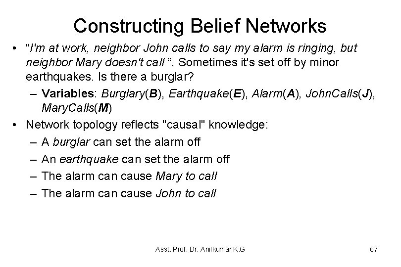
Constructing Belief Networks • “I'm at work, neighbor John calls to say my alarm is ringing, but neighbor Mary doesn't call “. Sometimes it's set off by minor earthquakes. Is there a burglar? – Variables: Burglary(B), Earthquake(E), Alarm(A), John. Calls(J), Mary. Calls(M) • Network topology reflects "causal" knowledge: – A burglar can set the alarm off – An earthquake can set the alarm off – The alarm can cause Mary to call – The alarm can cause John to call Asst. Prof. Dr. Anilkumar K. G 67

Constructing Belief Networks The topology shows that Burglary and Earthquake Directly affect the probability Of the alarm. But John. Call and Mary. Call depend on the Alarm. • In the CPT(conditional probability table), letters B, E, A, J and M stand for Burglary, Earthquake, Alarm, John. Calls and Mary. Calls respectively Asst. Prof. Dr. Anilkumar K. G 68

Constructing Belief Networks • Once we have specified the topology, we need to specify the CPT for each node. For example, the CPT for the random variable Alarm might look like this: B E T T F F T F P(A|B, E) T F 0. 95 0. 05 0. 94 0. 06 0. 29 0. 71 0. 001 0. 999 Asst. Prof. Dr. Anilkumar K. G 69

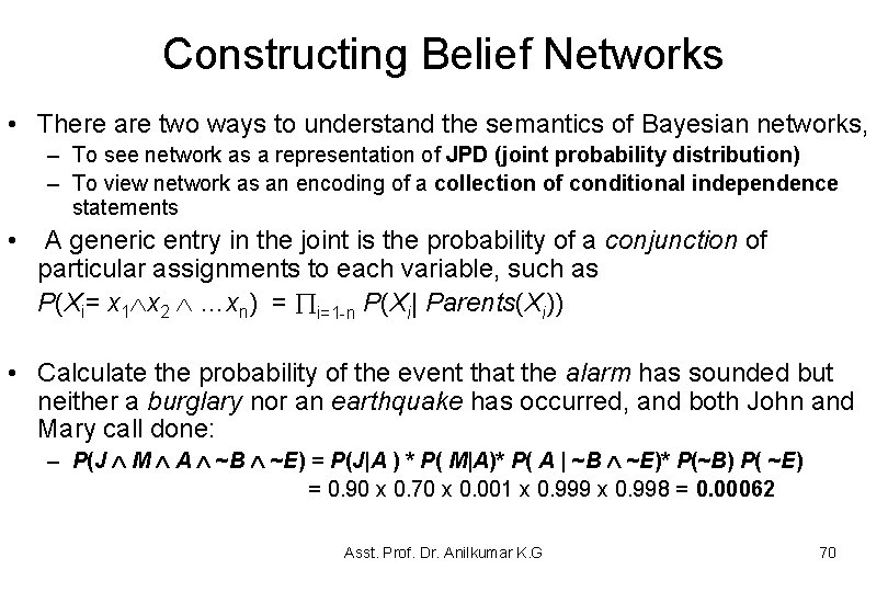
Constructing Belief Networks • There are two ways to understand the semantics of Bayesian networks, – To see network as a representation of JPD (joint probability distribution) – To view network as an encoding of a collection of conditional independence statements • A generic entry in the joint is the probability of a conjunction of particular assignments to each variable, such as P(Xi= x 1 x 2 …xn) = i=1 -n P(Xi| Parents(Xi)) • Calculate the probability of the event that the alarm has sounded but neither a burglary nor an earthquake has occurred, and both John and Mary call done: – P(J M A ~B ~E) = P(J|A ) * P( M|A)* P( A | ~B ~E)* P(~B) P( ~E) = 0. 90 x 0. 70 x 0. 001 x 0. 999 x 0. 998 = 0. 00062 Asst. Prof. Dr. Anilkumar K. G 70

Constructing Belief Networks • Example 8. 16 Consider the problem of diagnosing why someone is sneezing and perhaps has a fever. Sneezing could be because of influenza or because of hay fever. They are not independent, but are correlated due to the season. Suppose hay fever depends on the season because it depends on the amount of pollen, which in turn depends on the season. The agent does not get to observe sneezing directly, but rather observed just the “Achoo” sound. Suppose fever depends directly on influenza. These dependency considerations lead to the belief network of Figure 8. 4. Asst. Prof. Dr. Anilkumar K. G 71

Constructing Belief Networks Asst. Prof. Dr. Anilkumar K. G 72

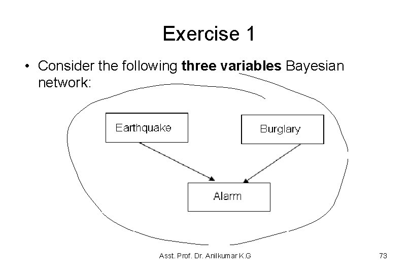
Exercise 1 • Consider the following three variables Bayesian network: Asst. Prof. Dr. Anilkumar K. G 73

Exercise 1 cont • The joint distribution over the three variables; Earthquake (E), Burglary (B) and Alarm (A) are shown below: Asst. Prof. Dr. Anilkumar K. G 74

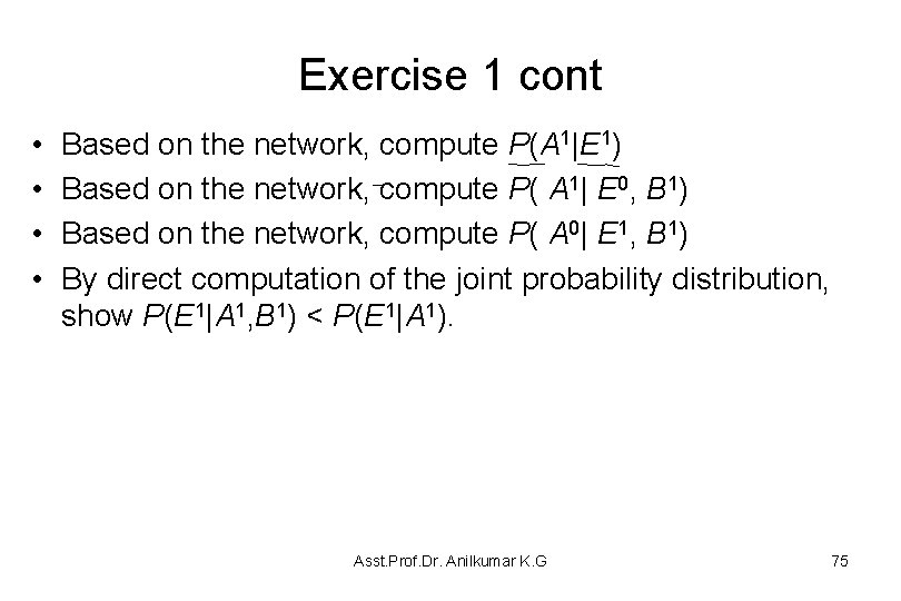
Exercise 1 cont • • Based on the network, compute P(A 1|E 1) Based on the network, compute P( A 1| E 0, B 1) Based on the network, compute P( A 0| E 1, B 1) By direct computation of the joint probability distribution, show P(E 1|A 1, B 1) < P(E 1|A 1). Asst. Prof. Dr. Anilkumar K. G 75

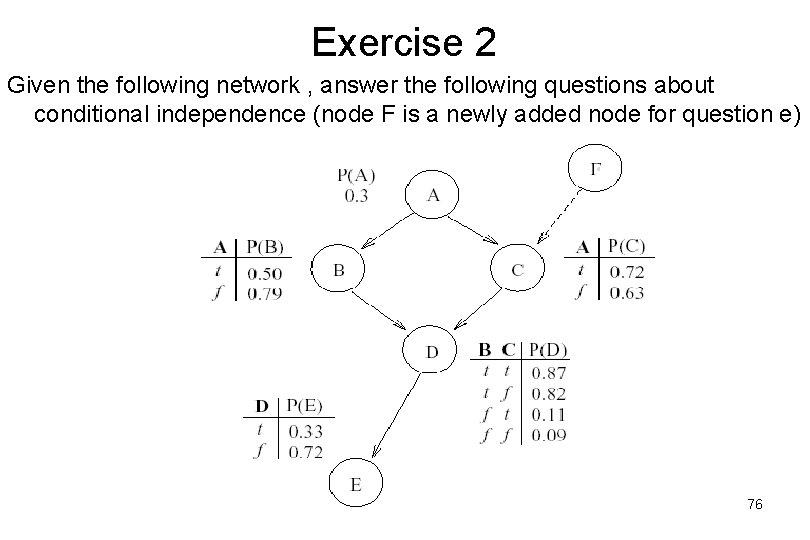
Exercise 2 Given the following network , answer the following questions about conditional independence (node F is a newly added node for question e) Asst. Prof. Dr. Anilkumar K. G 76

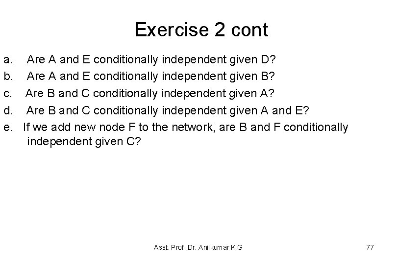
Exercise 2 cont a. Are A and E conditionally independent given D? b. Are A and E conditionally independent given B? c. Are B and C conditionally independent given A? d. Are B and C conditionally independent given A and E? e. If we add new node F to the network, are B and F conditionally independent given C? Asst. Prof. Dr. Anilkumar K. G 77

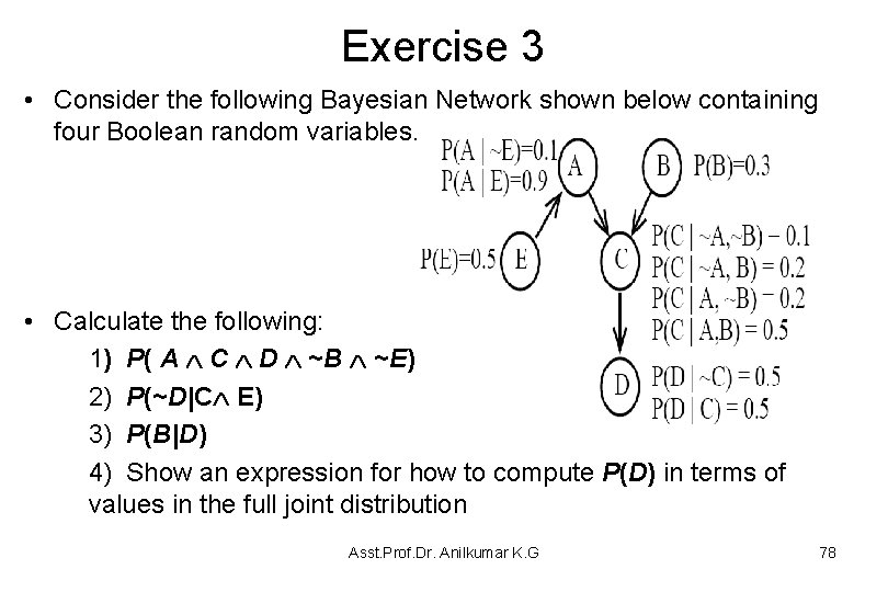
Exercise 3 • Consider the following Bayesian Network shown below containing four Boolean random variables. • Calculate the following: 1) P( A C D ~B ~E) 2) P(~D|C E) 3) P(B|D) 4) Show an expression for how to compute P(D) in terms of values in the full joint distribution Asst. Prof. Dr. Anilkumar K. G 78

Probabilistic Inference • Next Section Asst. Prof. Dr. Anilkumar K. G 79