Chapter 8 RandomVariate Generation Purpose Overview Inverse Transform

Chapter 8 Random-Variate Generation

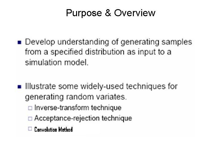
Purpose & Overview

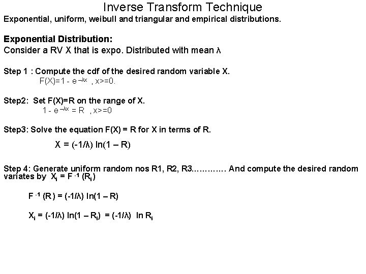
Inverse Transform Technique Exponential, uniform, weibull and triangular and empirical distributions. Exponential Distribution: Consider a RV X that is expo. Distributed with mean λ Step 1 : Compute the cdf of the desired random variable X. F(X)=1 - e –λx , x>=0. Step 2: Set F(X)=R on the range of X. 1 - e –λx = R , x>=0 Step 3: Solve the equation F(X) = R for X in terms of R. X = (-1/λ) ln(1 – R) Step 4: Generate uniform random nos R 1, R 2, R 3…………. And compute the desired random variates by Xi = F -1 (Ri ) F -1 (R ) = (-1/λ) ln(1 – R) Xi = (-1/λ) ln(1 – Ri) = (-1/λ) ln Ri

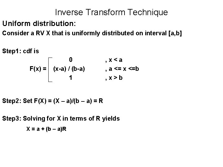
Inverse Transform Technique Uniform distribution: Consider a RV X that is uniformly distributed on interval [a, b] Step 1: cdf is F(x) = 0 (x-a) / (b-a) 1 , x<a , a <= x <=b , x>b Step 2: Set F(X) = (X – a)/(b – a) = R Step 3: Solving for X in terms of R yields X = a + (b – a)R

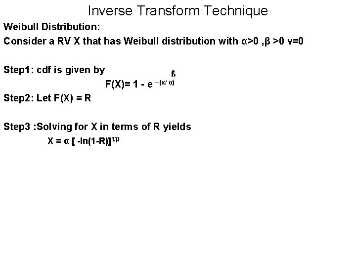
Inverse Transform Technique Weibull Distribution: Consider a RV X that has Weibull distribution with α>0 , β >0 v=0 Step 1: cdf is given by F(X)= 1 - e –(x/ α) Step 2: Let F(X) = R Step 3 : Solving for X in terms of R yields X = α [ -ln(1 -R)]1/β

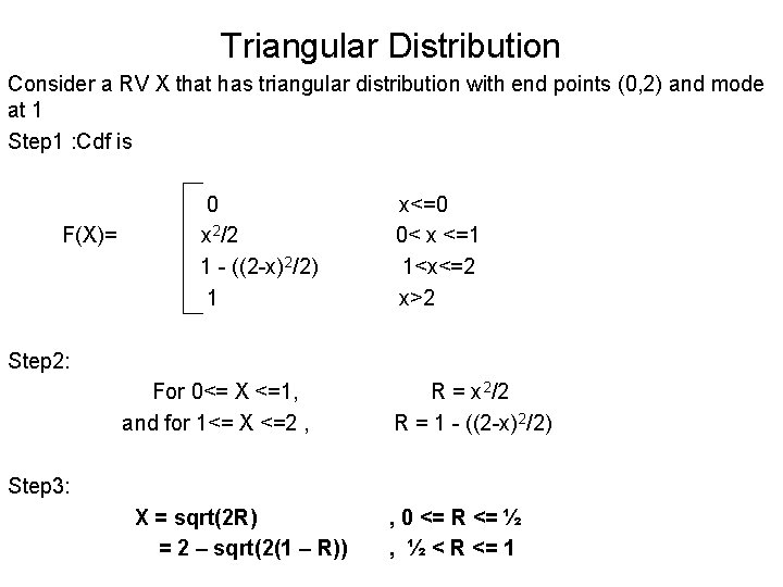
Triangular Distribution Consider a RV X that has triangular distribution with end points (0, 2) and mode at 1 Step 1 : Cdf is F(X)= 0 x 2/2 1 - ((2 -x)2/2) 1 x<=0 0< x <=1 1<x<=2 x>2 Step 2: For 0<= X <=1, and for 1<= X <=2 , R = x 2/2 R = 1 - ((2 -x) 2/2) Step 3: X = sqrt(2 R) = 2 – sqrt(2(1 – R)) , 0 <= R <= ½ , ½ < R <= 1

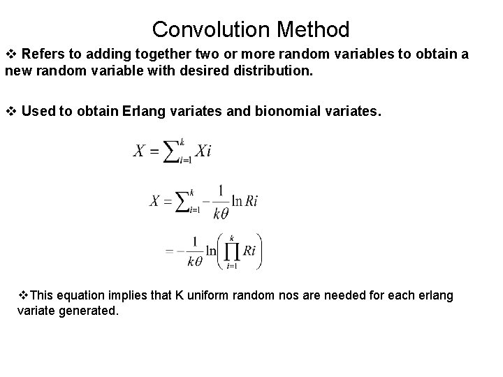
Convolution Method v Refers to adding together two or more random variables to obtain a new random variable with desired distribution. v Used to obtain Erlang variates and bionomial variates. v. This equation implies that K uniform random nos are needed for each erlang variate generated.

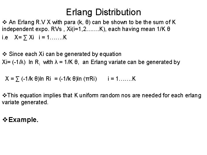
Erlang Distribution v An Erlang R. V X with para (k, θ) can be shown to be the sum of K independent expo. RVs , Xi(i=1, 2……. K), each having mean 1/K θ i. e X= ∑ Xi i = 1……. K v Since each Xi can be generated by equation Xi= (-1/λ) ln Ri with λ = 1/K θ, an Erlang variate can be generated by X = ∑ (-1/k θ)ln Ri = (-1/k θ)ln (πRi) i = 1……. K v. This equation implies that K uniform random nos are needed for each erlang variate generated. v. Example.

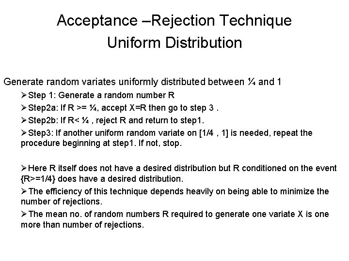
Acceptance –Rejection Technique Uniform Distribution Generate random variates uniformly distributed between ¼ and 1 ØStep 1: Generate a random number R ØStep 2 a: If R >= ¼, accept X=R then go to step 3. ØStep 2 b: If R< ¼ , reject R and return to step 1. ØStep 3: If another uniform random variate on [1/4 , 1] is needed, repeat the procedure beginning at step 1. If not, stop. ØHere R itself does not have a desired distribution but R conditioned on the event {R>=1/4} does have a desired distribution. ØThe efficiency of this technique depends heavily on being able to minimize the number of rejections. ØThe mean no. of random numbers R required to generate one variate X is one more than number of rejections.

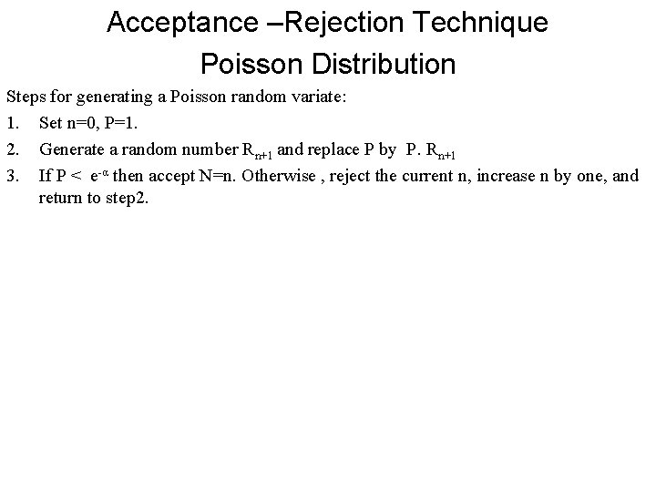
Acceptance –Rejection Technique Poisson Distribution Steps for generating a Poisson random variate: 1. Set n=0, P=1. 2. Generate a random number Rn+1 and replace P by P. Rn+1 3. If P < e-α then accept N=n. Otherwise , reject the current n, increase n by one, and return to step 2.

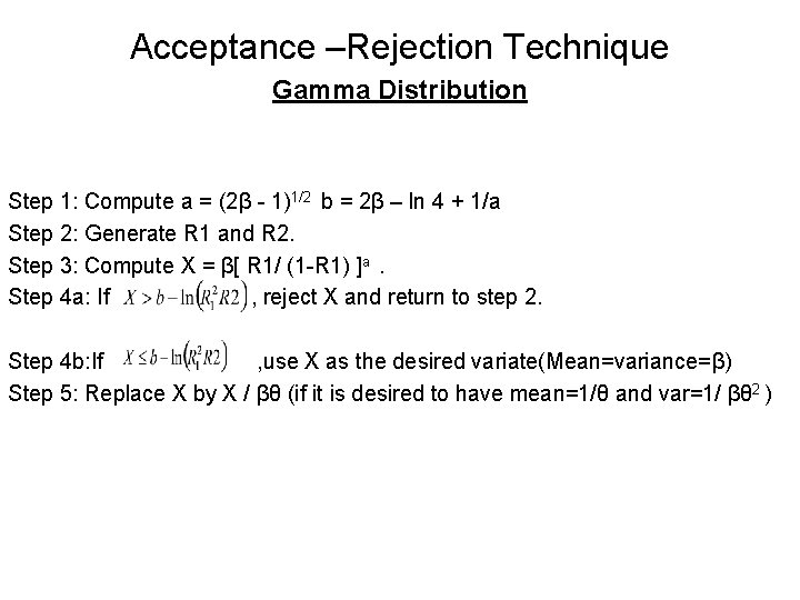
Acceptance –Rejection Technique Gamma Distribution Step 1: Compute a = (2β - 1)1/2 b = 2β – ln 4 + 1/a Step 2: Generate R 1 and R 2. Step 3: Compute X = β[ R 1/ (1 -R 1) ]a. Step 4 a: If , reject X and return to step 2. Step 4 b: If , use X as the desired variate(Mean=variance=β) Step 5: Replace X by X / βθ (if it is desired to have mean=1/θ and var=1/ βθ 2 )