Chapter 8 Production Theory and Analysis The Theory

Chapter 8 Production Theory and Analysis

The Theory and Estimation of Production • The Production Function • COBB–DOUGLAS PRODUCTION FUNCTION • Production in the Short Run • • Total, Average, and Marginal Product Law of Diminishing Returns Stages of Production Optimal Input Usage • Production in the Long Run • Returns to Scale

Production • Production is the creation of goods and services from inputs or resources, such as labour, machinery and other capital equipment, land, raw materials, and so on.

The Production Function • A production function defines the relationship between inputs and the maximum amount that can be produced within a given time period with a given technology. • Technically efficient (max. output) vs. Technically inefficient • Economic efficiency (min. cost)

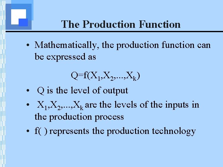
The Production Function • Mathematically, the production function can be expressed as Q=f(X 1, X 2, . . . , Xk) • Q is the level of output • X 1, X 2, . . . , Xk are the levels of the inputs in the production process • f( ) represents the production technology

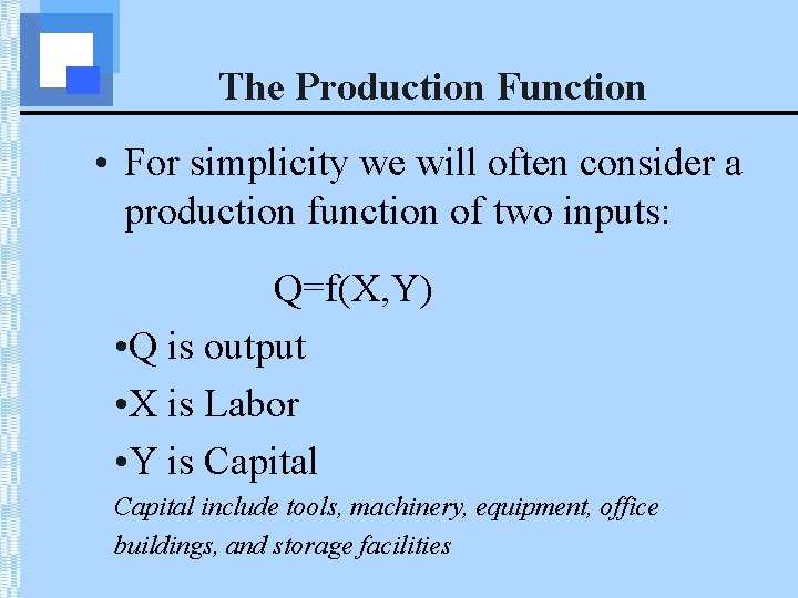
The Production Function • For simplicity we will often consider a production function of two inputs: Q=f(X, Y) • Q is output • X is Labor • Y is Capital include tools, machinery, equipment, office buildings, and storage facilities

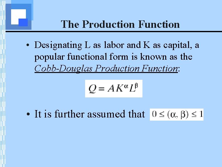
The Production Function • Designating L as labor and K as capital, a popular functional form is known as the Cobb-Douglas Production Function: • It is further assumed that

Properties of Production Functiona • Substitutability • Returns to Scale • Constant Returns to Scale (CRTS) • Increasing Returns to Scale (IRTS) • Decreasing Returns to Scale (DRTS) • Law of Diminishing Marginal Product

The Production Function • When discussing production, it is important to distinguish between two time frames. • The short-run production function describes the maximum quantity of good or service that can be produced by a set of inputs, assuming that at least one of the inputs is fixed at some level.

The Production Function • The long-run production function describes the maximum quantity of good or service that can be produced by a set of inputs, assuming that the firm is free to adjust the level of all inputs.

Returns to Input • The production function is also referred to as the total product function • The increase in production due to an increase in input (such as labour) is called returns to the input (such as returns to labour) • Generally the first few inputs are highly productive, but additional units are less productive (e. g. : computer programmers working in a small room) 11

Q Example: Production as workers increase Each Additional worker Is equally productive Each Additional worker Is more productive Each Additional worker Is less productive Each Additional worker Decreases Production Total Product L 12

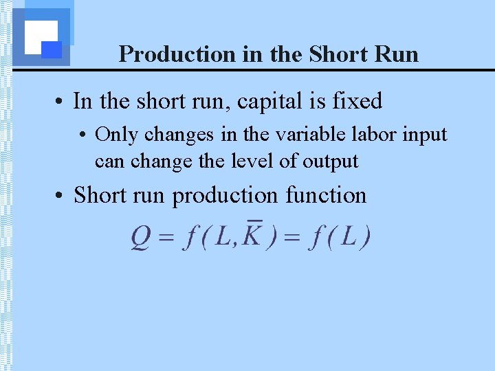
Production in the Short Run • In the short run, capital is fixed • Only changes in the variable labor input can change the level of output • Short run production function

Production in the Short Run • When discussing production in the short run, three definitions are important. • Total Product • Marginal Product • Average Product

Production in the Short Run • Total product (TP) is another name for output in the short run. The total product function is the same as the short run production function.

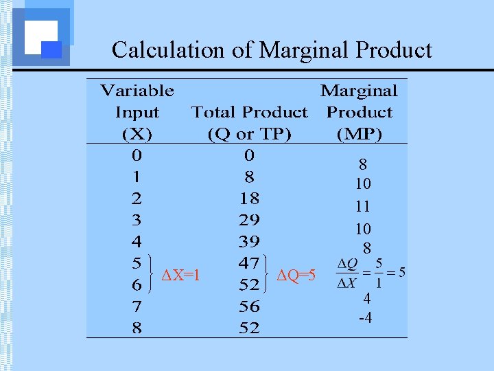
Production in the Short Run • The marginal product (MP) of a variable input is the change in output (or TP) resulting from a one unit change in the input (resource). • MP tells us how output changes as we change the level of the input by one unit.

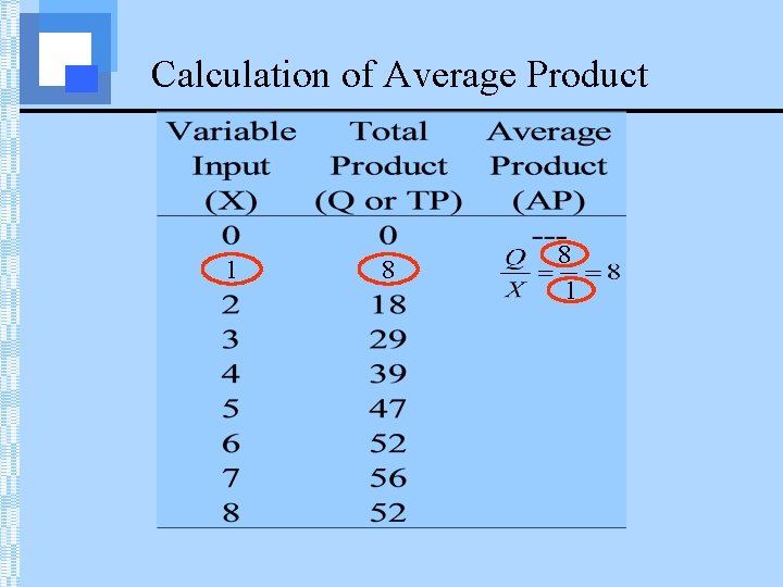
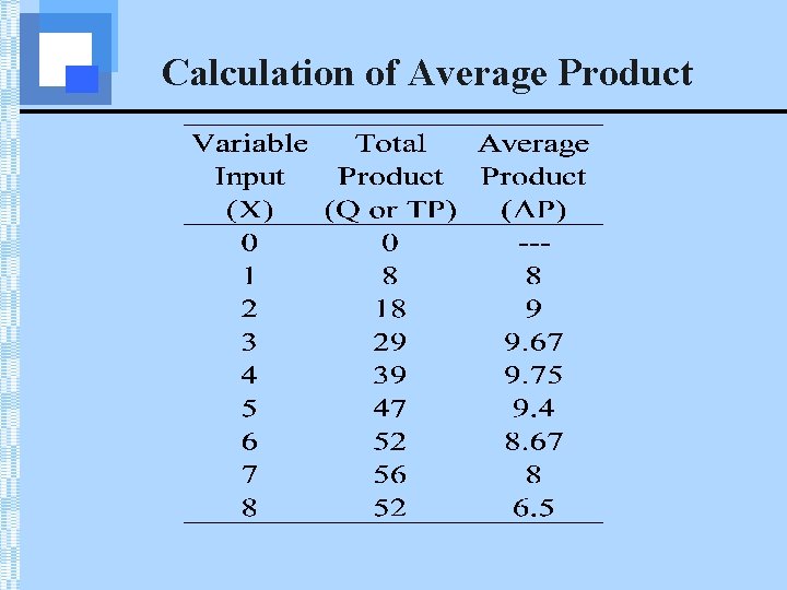
Production in the Short Run • The average product (AP) of an input is the total product divided by the level of the input. • AP tells us, on average, how many units of output are produced per unit of input used.

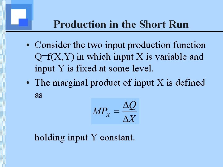
Production in the Short Run • Consider the two input production function Q=f(X, Y) in which input X is variable and input Y is fixed at some level. • The marginal product of input X is defined as holding input Y constant.

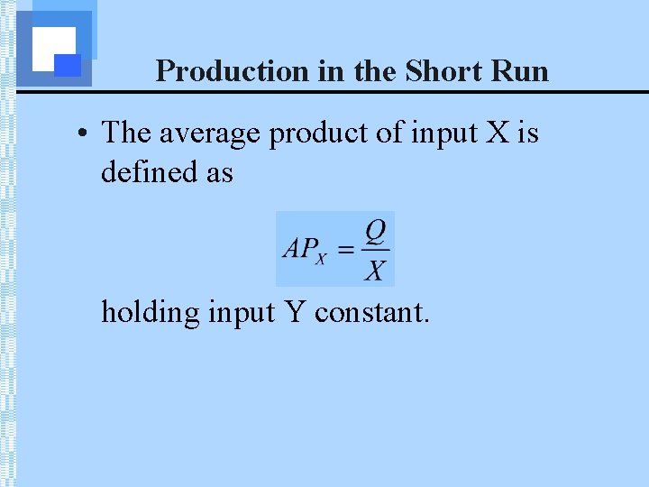
Production in the Short Run • The average product of input X is defined as holding input Y constant.

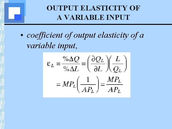
OUTPUT ELASTICITY OF A VARIABLE INPUT • coefficient of output elasticity of a variable input,

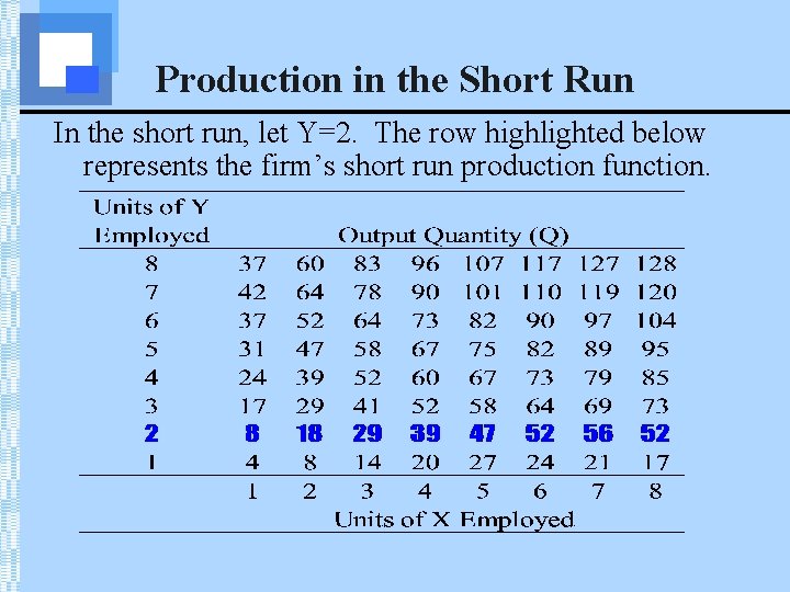
Production in the Short Run The table below represents a firm’s production function, Q=f(X, Y):

Production in the Short Run In the short run, let Y=2. The row highlighted below represents the firm’s short run production function.

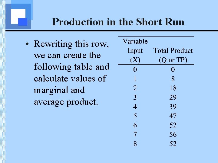
Production in the Short Run • Rewriting this row, we can create the following table and calculate values of marginal and average product.

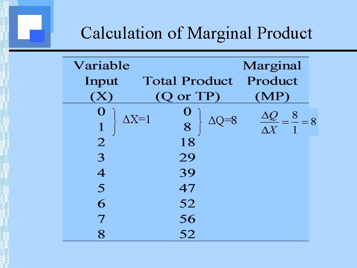
Calculation of Marginal Product ΔX=1 ΔQ=8

Calculation of Marginal Product 8 10 11 10 8 ΔX=1 ΔQ=5 4 -4

Calculation of Average Product 1 8 8 1

Calculation of Average Product

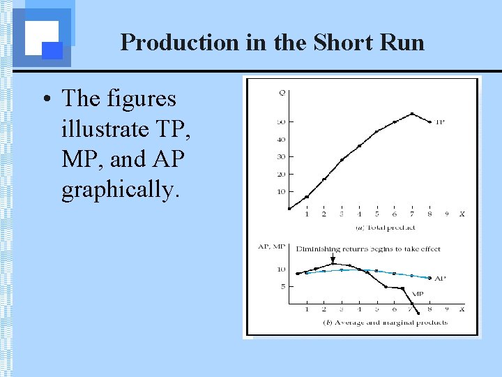
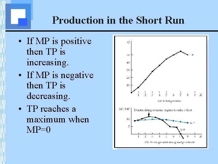
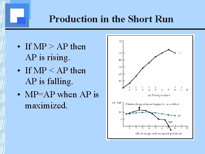
Production in the Short Run • The figures illustrate TP, MP, and AP graphically.

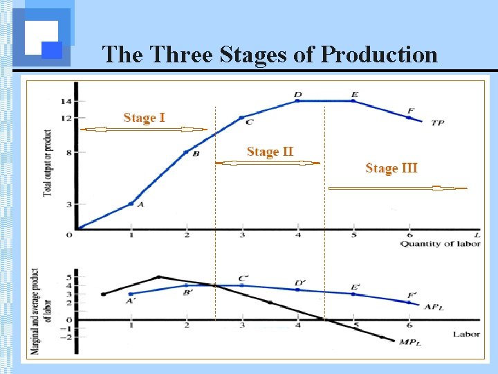
Production in the Short Run • If MP is positive then TP is increasing. • If MP is negative then TP is decreasing. • TP reaches a maximum when MP=0

Production in the Short Run • If MP > AP then AP is rising. • If MP < AP then AP is falling. • MP=AP when AP is maximized.

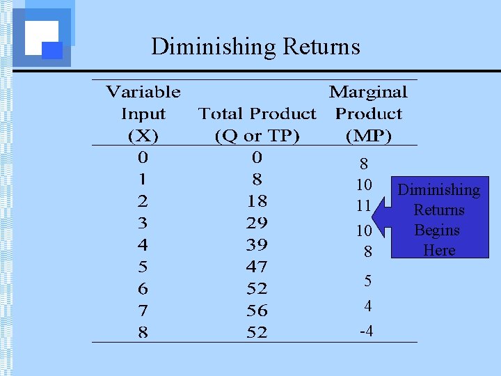
The Law of Diminishing Returns • Definition • As additional units of a variable input are combined with a fixed input, at some point the additional output (i. e. , marginal product) starts to diminish.

Diminishing Returns 8 10 11 10 8 5 4 -4 Diminishing Returns Begins Here

The Law of Diminishing Returns • Reasons Increasing Returns Teamwork and Specialization MP Diminishing Returns Begins Fewer opportunities for teamwork and specialization X MP

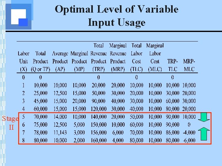
The Three Stages of Production • Stage I • From zero units of the variable input to where AP is maximized • Stage II • From the maximum AP to where MP=0 • Stage III • From where MP=0 on

The Three Stages of Production

The Three Stages of Production • In the short run, rational firms should only be operating in Stage II. • Why Stage II? • Why not Stage III? • Firm uses more variable inputs to produce less output! • Why not Stage I? • Underutilizing fixed capacity. • Can increase output per unit by increasing the amount of the variable input.

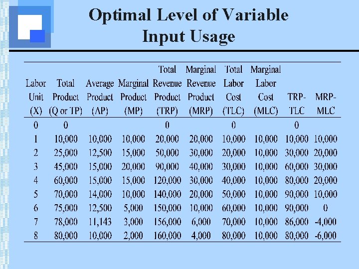
Optimal Level of Variable Input Usage • Consider the following short run production process. Where is Stage II?

Optimal Level of Variable Input Usage Stage II

Optimal Level of Variable Input Usage • What level of input usage within Stage II is best for the firm? • The answer depends upon how many units of output the firm can sell, the price of the product, and the monetary costs of employing the variable input.

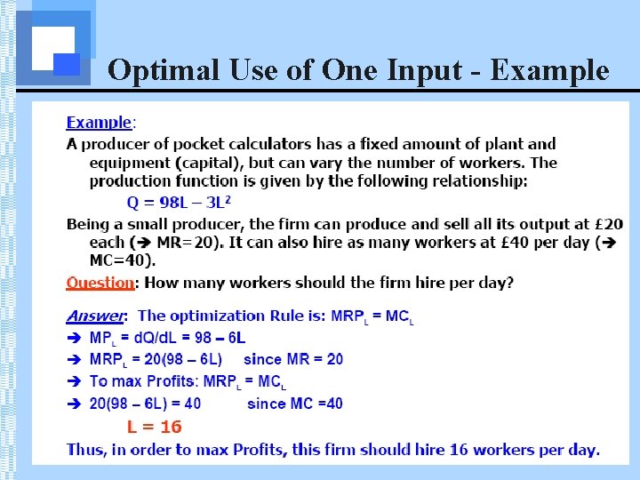
Optimal Level of Variable Input Usage • A profit-maximizing firm operating in perfectly competitive output and input markets will be using the optimal amount of an input at the point at which the monetary value of the input’s marginal revenue product is equal to the additional cost of using that input. • Where MRP=MLC.

Optimal Level of Variable Input Usage • In order to determine the optimal input usage we assume that the firm operates in a perfectly competitive market for its input and its output. • Product price, P=$2 • Variable input price, w=$10, 000

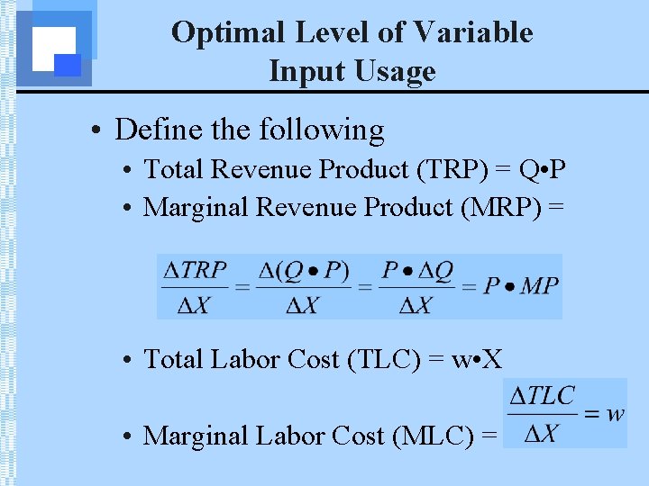
Optimal Level of Variable Input Usage • Define the following • Total Revenue Product (TRP) = Q • P • Marginal Revenue Product (MRP) = • Total Labor Cost (TLC) = w • X • Marginal Labor Cost (MLC) =

Optimal Level of Variable Input Usage

Optimal Level of Variable Input Usage Stage II

Optimal Use of One Input - Example

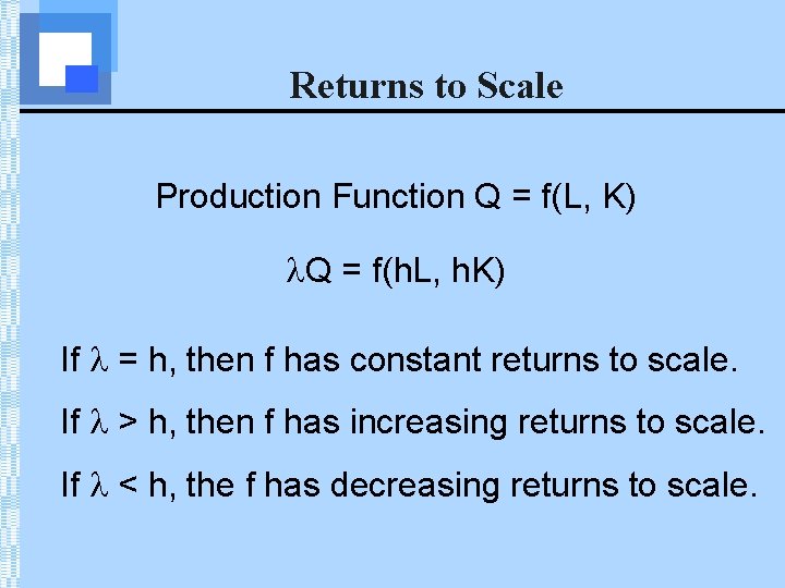
Production in the Long Run • In the long run, all inputs are variable. • The long run production process is described by the concept of returns to scale. • Returns to scale describes what happens to total output as all of the inputs are changed by the same proportion.

Returns to Scale Production Function Q = f(L, K) Q = f(h. L, h. K) If = h, then f has constant returns to scale. If > h, then f has increasing returns to scale. If < h, the f has decreasing returns to scale.

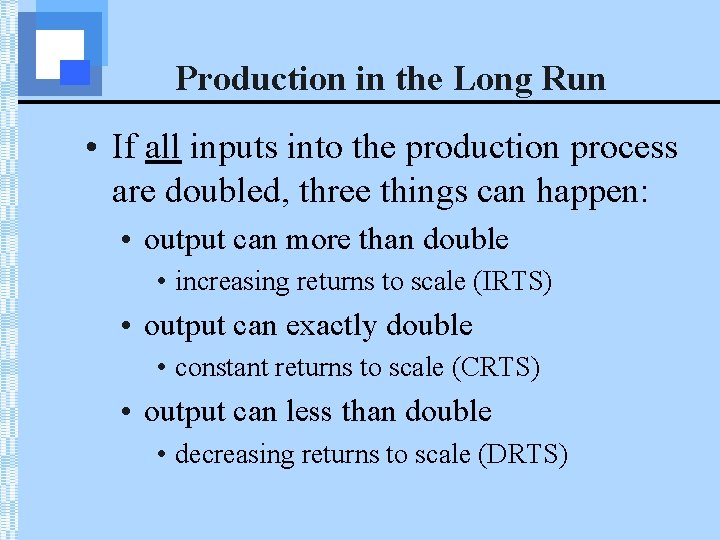
Production in the Long Run • If all inputs into the production process are doubled, three things can happen: • output can more than double • increasing returns to scale (IRTS) • output can exactly double • constant returns to scale (CRTS) • output can less than double • decreasing returns to scale (DRTS)

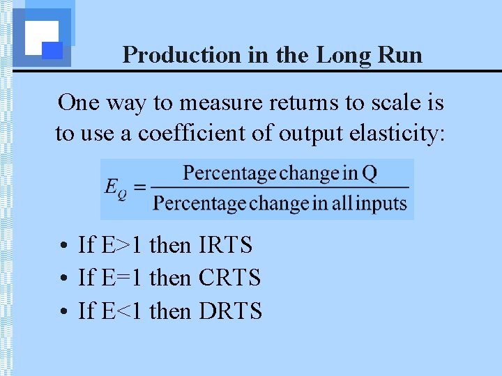
Production in the Long Run One way to measure returns to scale is to use a coefficient of output elasticity: • If E>1 then IRTS • If E=1 then CRTS • If E<1 then DRTS

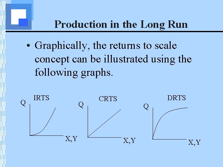
Production in the Long Run • Graphically, the returns to scale concept can be illustrated using the following graphs. Q IRTS Q X, Y DRTS CRTS Q X, Y

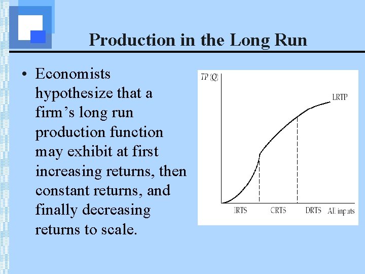
Production in the Long Run • Economists hypothesize that a firm’s long run production function may exhibit at first increasing returns, then constant returns, and finally decreasing returns to scale.

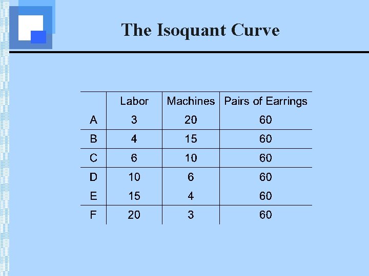
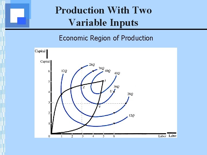
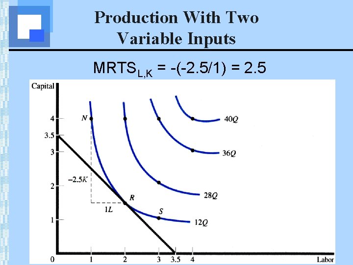
Production Isoquants • In the long run, all inputs are variable & isoquants are used to study production decisions • An isoquant is a curve showing all possible input combinations capable of producing a given level of output • Isoquants are downward sloping; if greater amounts of labor are used, less capital is required to produce a given output • Firms will only use combinations of two inputs that are in the economic region of production, which is defined by the portion of each isoquant that is negatively sloped.

The Isoquant Curve

The Isoquant Curve

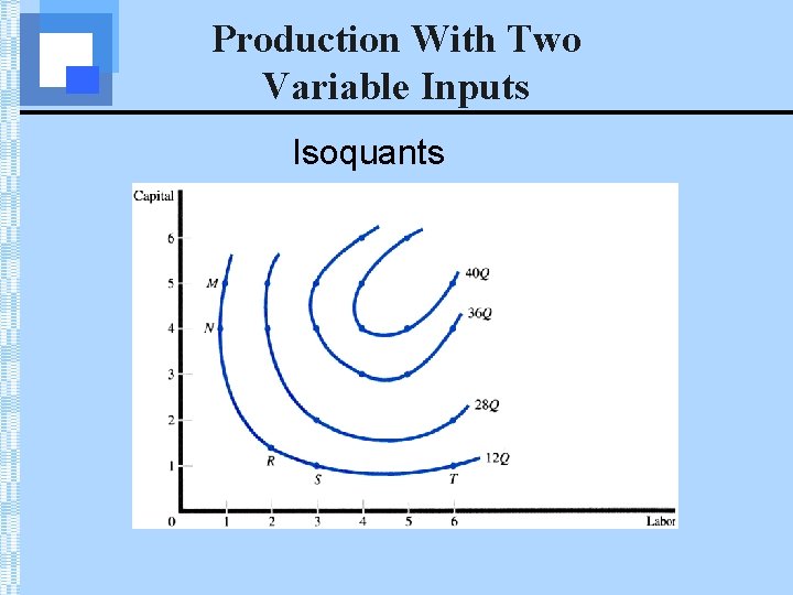
Production With Two Variable Inputs Isoquants

Production With Two Variable Inputs Economic Region of Production

Properties of Isoquant • Isoquants further from the origin represent greater output levels • Isoquants slope down to the right • Isoquants do not intersect • Isoquants are usually convex to the origin

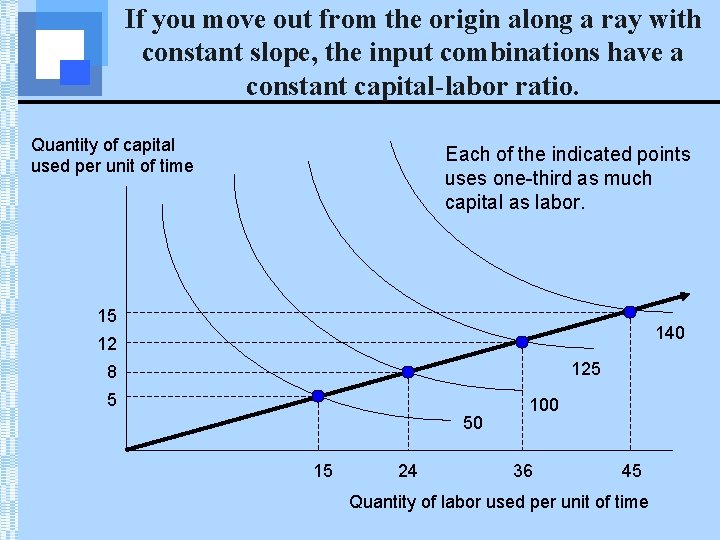
If you move out from the origin along a ray with constant slope, the input combinations have a constant capital-labor ratio. Quantity of capital used per unit of time Each of the indicated points uses one-third as much capital as labor. 15 140 12 125 8 5 50 15 24 100 36 45 Quantity of labor used per unit of time

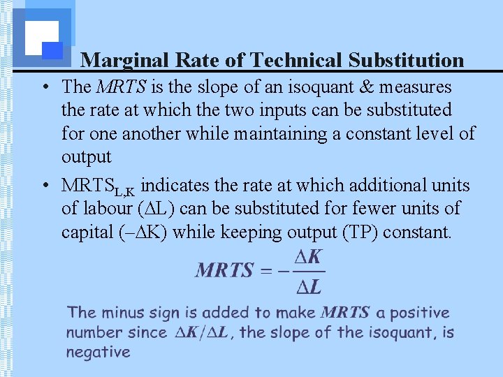
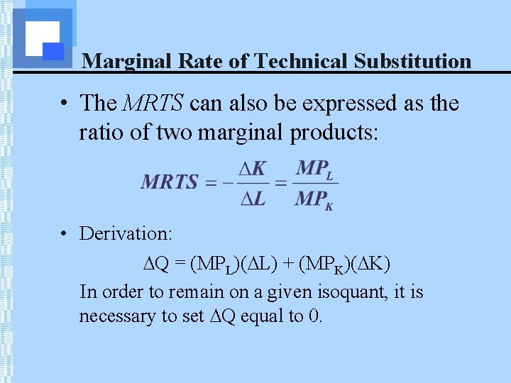
Marginal Rate of Technical Substitution • The MRTS is the slope of an isoquant & measures the rate at which the two inputs can be substituted for one another while maintaining a constant level of output • MRTSL, K indicates the rate at which additional units of labour (∆L) can be substituted for fewer units of capital (–∆K) while keeping output (TP) constant.

Production With Two Variable Inputs MRTSL, K = -(-2. 5/1) = 2. 5

Marginal Rate of Technical Substitution • The MRTS can also be expressed as the ratio of two marginal products: • Derivation: ∆Q = (MPL)(∆L) + (MPK)(∆K) In order to remain on a given isoquant, it is necessary to set ∆Q equal to 0.

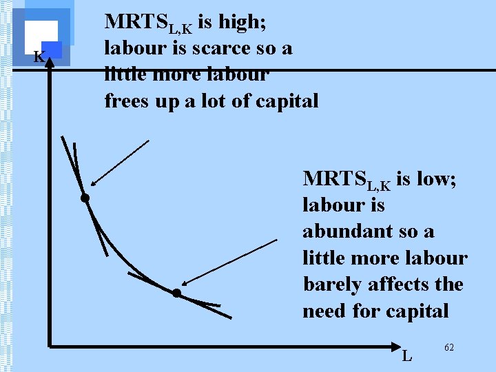
MRTSL, K is high; labour is scarce so a little more labour frees up a lot of capital K • • MRTSL, K is low; labour is abundant so a little more labour barely affects the need for capital L 62

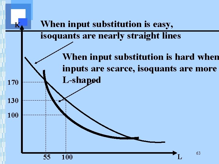
K When input substitution is easy, isoquants are nearly straight lines When input substitution is hard when inputs are scarce, isoquants are more L-shaped 170 130 100 55 100 L 63

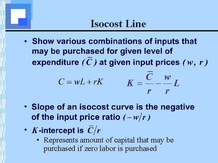
Isocost Line • • Represents amount of capital that may be purchased if zero labor is purchased

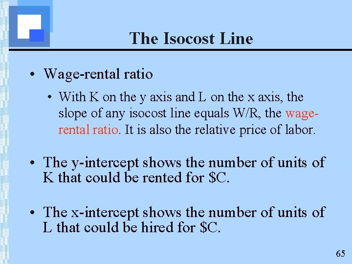
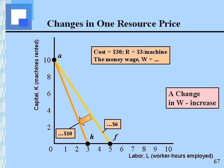
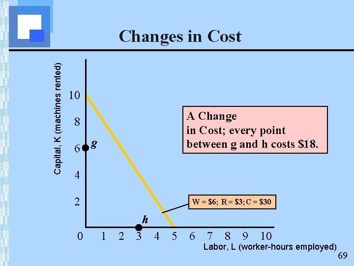
The Isocost Line • Wage-rental ratio • With K on the y axis and L on the x axis, the slope of any isocost line equals W/R, the wagerental ratio. It is also the relative price of labor. • The y-intercept shows the number of units of K that could be rented for $C. • The x-intercept shows the number of units of L that could be hired for $C. 65

Capital, K (machines rented) Changes in One Resource Price 10 Cost = $30; R = $3/machine The money wage, W =. . . a 8 6 A Change in W - increase 4 2 0 …$6 …$10 1 h 2 3 f 4 5 6 7 8 9 10 Labor, L (worker-hours employed) 67

Capital, K (machines rented) Changes in Cost 10 A Change in Cost; every point between g and h costs $18. 8 6 g 4 2 W = $6; R = $3; C = $30 h 0 1 2 3 4 5 6 7 8 9 10 Labor, L (worker-hours employed) 69

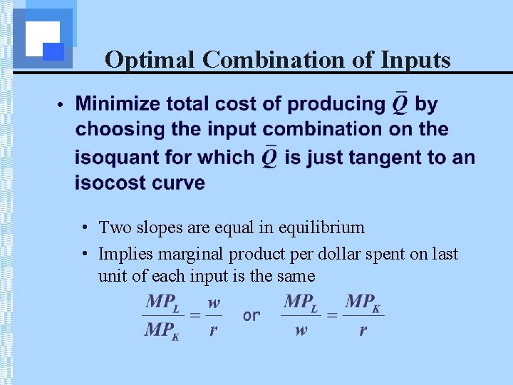
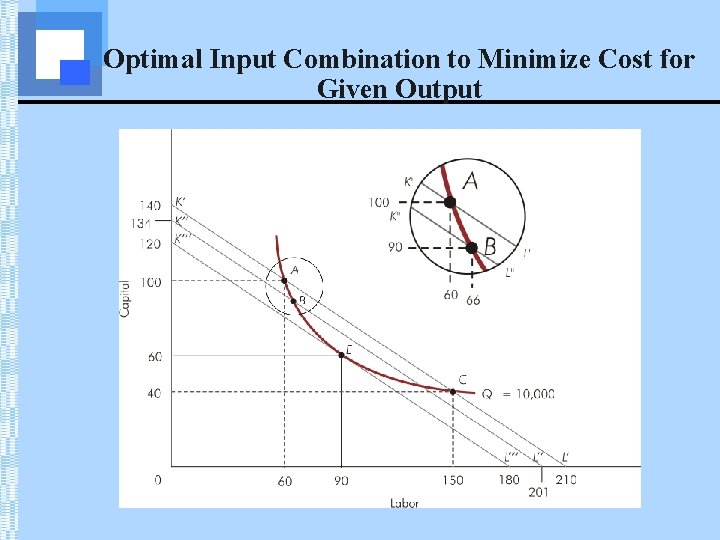
Optimal Combination of Inputs • • Two slopes are equal in equilibrium • Implies marginal product per dollar spent on last unit of each input is the same

Optimal Input Combination to Minimize Cost for Given Output

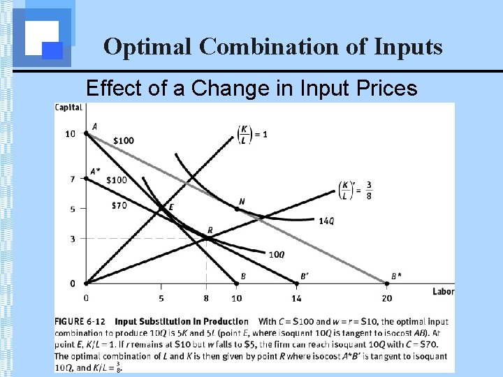
Optimal Combination of Inputs Effect of a Change in Input Prices

Optimization & Cost • Expansion path gives the efficient (leastcost) input combinations for every level of output • Derived for a specific set of input prices • Along expansion path, input-price ratio is constant & equal to the marginal rate of technical substitution

Expansion Path