Chapter 8 Principles of Corporate Finance Tenth Edition

Chapter 8 Principles of Corporate Finance Tenth Edition Portfolio Theory and the Capital Asset Model Pricing Slides by Matthew Will Mc. Graw-Hill/Irwin Copyright © 2011 by the Mc. Graw-Hill Companies, Inc. All rights reserved.

Topics Covered Ø Harry Markowitz And The Birth Of Portfolio Theory Ø The Relationship Between Risk and Return Ø Validity and the Role of the CAPM Ø Some Alternative Theories 8 -2

Markowitz Portfolio Theory Ø Combining stocks into portfolios can reduce standard deviation, below the level obtained from a simple weighted average calculation. Ø Correlation coefficients make this possible. Ø The various weighted combinations of stocks that create this standard deviations constitute the set of efficient portfolios 8 -3

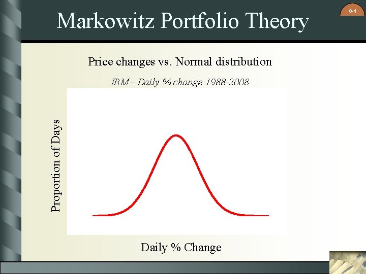
Markowitz Portfolio Theory Price changes vs. Normal distribution Proportion of Days IBM - Daily % change 1988 -2008 Daily % Change 8 -4

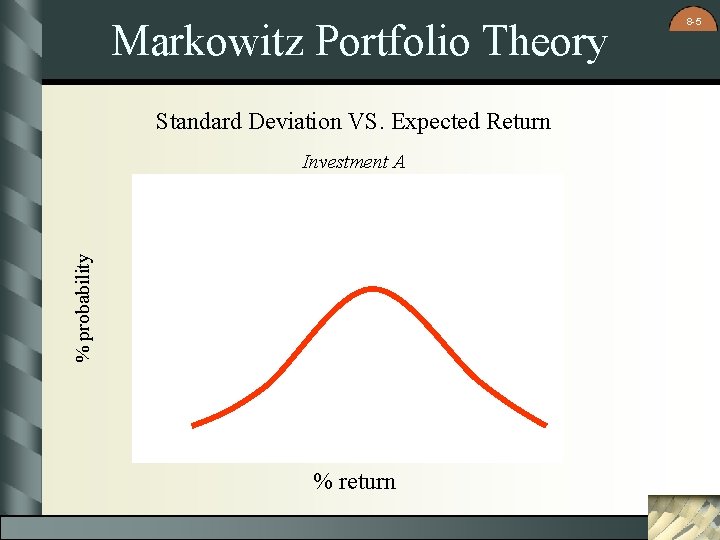
Markowitz Portfolio Theory Standard Deviation VS. Expected Return % probability Investment A % return 8 -5

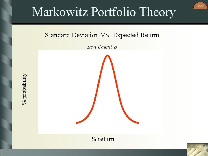
Markowitz Portfolio Theory Standard Deviation VS. Expected Return % probability Investment B % return 8 -6

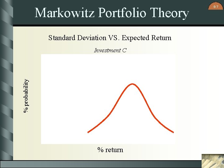
Markowitz Portfolio Theory Standard Deviation VS. Expected Return % probability Investment C % return 8 -7

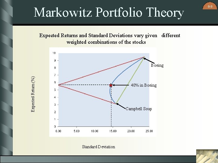
Markowitz Portfolio Theory Expected Returns and Standard Deviations vary given different weighted combinations of the stocks Expected Return (%) Boeing 40% in Boeing Campbell Soup Standard Deviation 8 -8

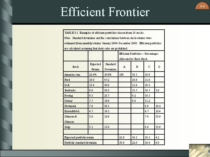
8 -9 Efficient Frontier TABLE 8. 1 Examples of efficient portfolios chosen from 10 stocks. Note: Standard deviations and the correlations between stock returns were estimated from monthly returns January 2004 -December 2008. Efficient portfolios are calculated assuming that short sales are prohibited. Efficient Portfolios – Percentages Allocated to Each Stock Expected Standard Return Deviation Amazon. com 22. 8% 50. 9% Ford 19. 0 Dell A 100 B C D 19. 1 10. 9 47. 2 19. 9 11. 0 13. 4 30. 9 15. 6 10. 3 Starbucks 9. 0 30. 3 13. 7 10. 7 Boeing 9. 5 23. 7 9. 2 10. 5 Disney 7. 7 19. 6 8. 8 11. 2 Newmont 7. 0 36. 1 9. 9 10. 2 Exxon. Mobil 4. 7 19. 1 9. 7 18. 4 Johnson & 3. 8 12. 6 7. 4 33. 9 3. 1 15. 8 8. 4 33. 9 3. 6 Johnson Soup Expected portfolio return 22. 8 14. 1 10. 5 4. 2 Portfolio standard deviation 50. 9 22. 0 16. 0 8. 8

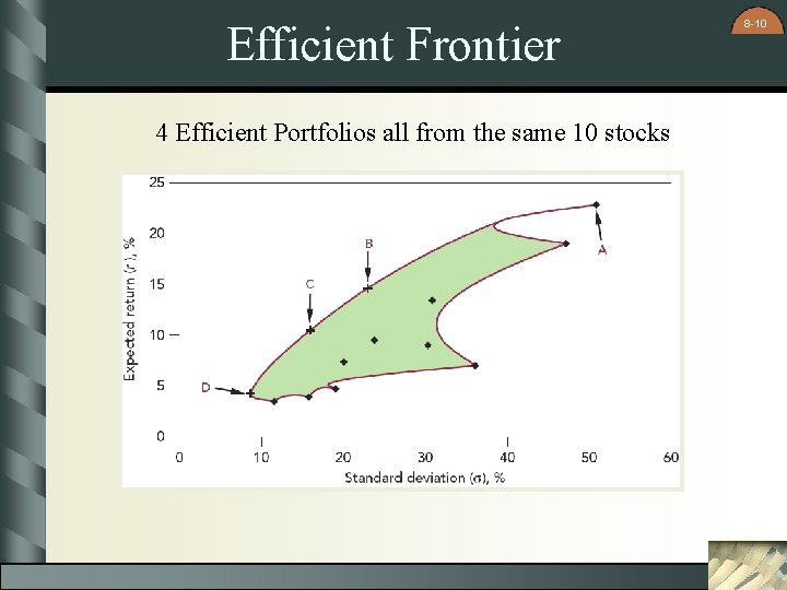
Efficient Frontier 4 Efficient Portfolios all from the same 10 stocks 8 -10

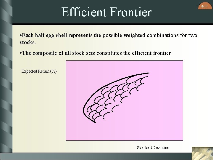
Efficient Frontier • Each half egg shell represents the possible weighted combinations for two stocks. • The composite of all stock sets constitutes the efficient frontier Expected Return (%) Standard Deviation 8 -11

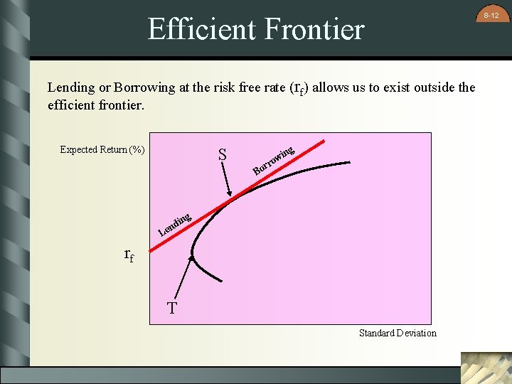
Efficient Frontier Lending or Borrowing at the risk free rate (rf) allows us to exist outside the efficient frontier. Expected Return (%) S ing w rro Bo g in nd e L rf T Standard Deviation 8 -12

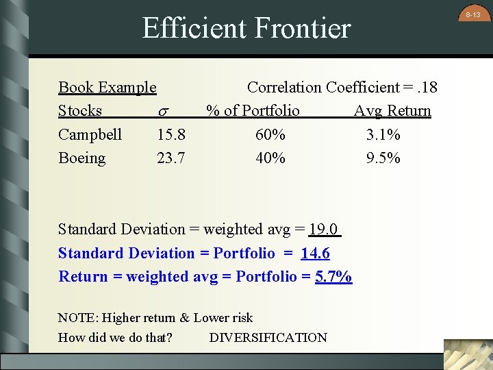
Efficient Frontier Book Example Stocks s Campbell 15. 8 Boeing 23. 7 Correlation Coefficient =. 18 % of Portfolio Avg Return 60% 3. 1% 40% 9. 5% Standard Deviation = weighted avg = 19. 0 Standard Deviation = Portfolio = 14. 6 Return = weighted avg = Portfolio = 5. 7% NOTE: Higher return & Lower risk How did we do that? DIVERSIFICATION 8 -13

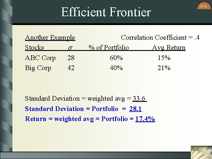
Efficient Frontier Another Example Stocks s ABC Corp 28 Big Corp 42 Correlation Coefficient =. 4 % of Portfolio Avg Return 60% 15% 40% 21% Standard Deviation = weighted avg = 33. 6 Standard Deviation = Portfolio = 28. 1 Return = weighted avg = Portfolio = 17. 4% 8 -14

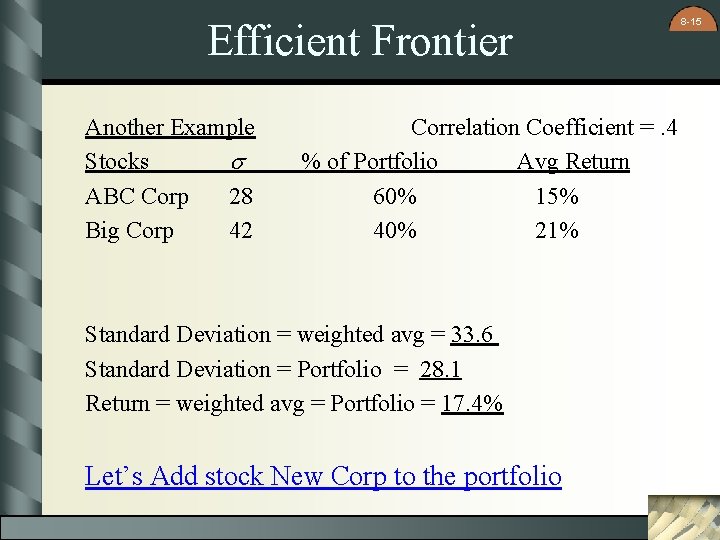
Efficient Frontier Another Example Stocks s ABC Corp 28 Big Corp 42 Correlation Coefficient =. 4 % of Portfolio Avg Return 60% 15% 40% 21% Standard Deviation = weighted avg = 33. 6 Standard Deviation = Portfolio = 28. 1 Return = weighted avg = Portfolio = 17. 4% Let’s Add stock New Corp to the portfolio 8 -15

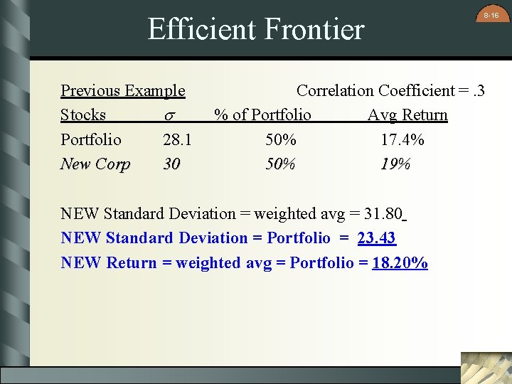
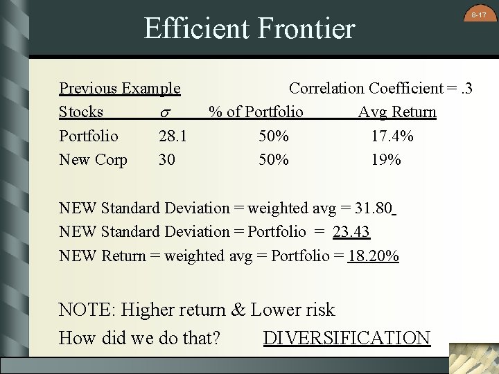
Efficient Frontier Previous Example Stocks s Portfolio 28. 1 New Corp 30 8 -16 Correlation Coefficient =. 3 % of Portfolio Avg Return 50% 17. 4% 50% 19% NEW Standard Deviation = weighted avg = 31. 80 NEW Standard Deviation = Portfolio = 23. 43 NEW Return = weighted avg = Portfolio = 18. 20%

Efficient Frontier Previous Example Stocks s Portfolio 28. 1 New Corp 30 8 -17 Correlation Coefficient =. 3 % of Portfolio Avg Return 50% 17. 4% 50% 19% NEW Standard Deviation = weighted avg = 31. 80 NEW Standard Deviation = Portfolio = 23. 43 NEW Return = weighted avg = Portfolio = 18. 20% NOTE: Higher return & Lower risk How did we do that? DIVERSIFICATION

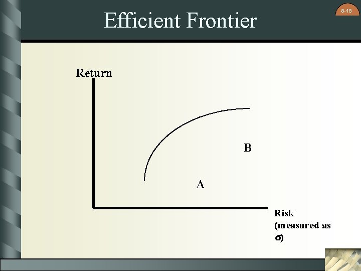
8 -18 Efficient Frontier Return B A Risk (measured as s)

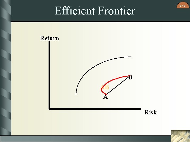
8 -19 Efficient Frontier Return B AB A Risk

8 -20 Efficient Frontier Return AB A N B Risk

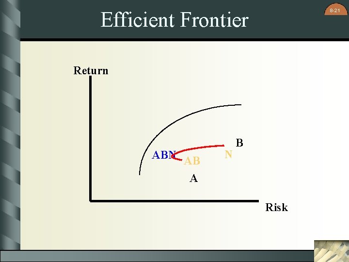
8 -21 Efficient Frontier Return ABN AB A N B Risk

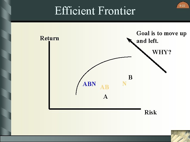
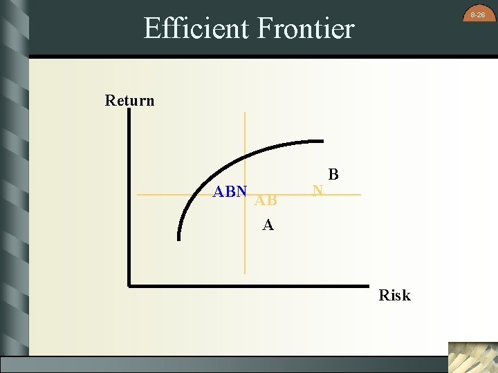
8 -22 Efficient Frontier Goal is to move up and left. Return WHY? ABN AB A N B Risk

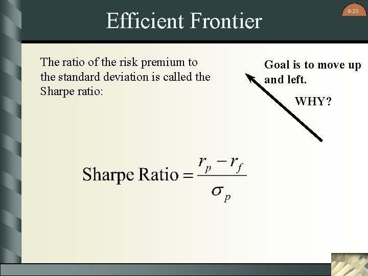
8 -23 Efficient Frontier The ratio of the risk premium to the standard deviation is called the Sharpe ratio: Goal is to move up and left. WHY?

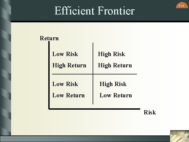
8 -24 Efficient Frontier Return Low Risk High Return Low Risk High Risk Low Return Risk

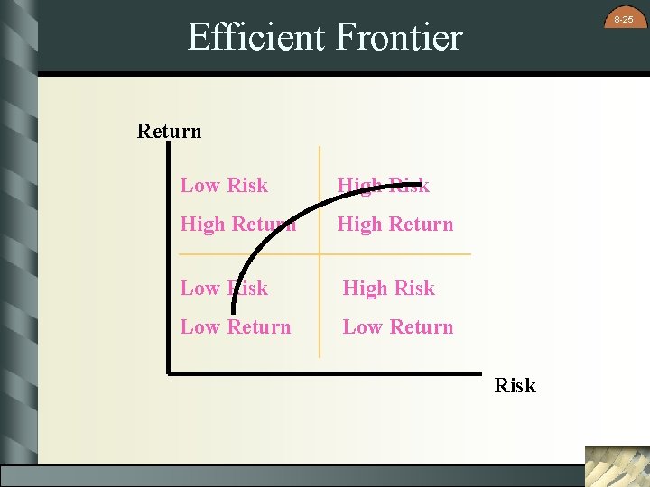
8 -25 Efficient Frontier Return Low Risk High Return Low Risk High Risk Low Return Risk

8 -26 Efficient Frontier Return ABN AB A N B Risk

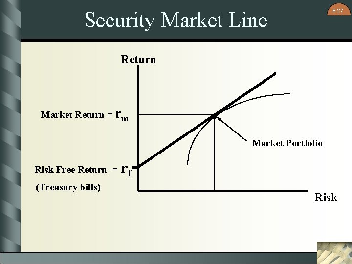
8 -27 Security Market Line Return Market Return = rm . Market Portfolio Risk Free Return = (Treasury bills) rf Risk

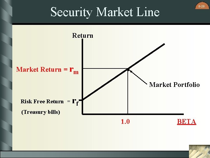
8 -28 Security Market Line Return Market Return = rm . Market Portfolio Risk Free Return = rf (Treasury bills) 1. 0 BETA

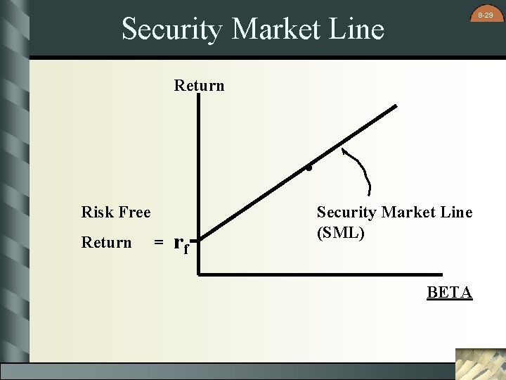
8 -29 Security Market Line Return . Risk Free Return = rf Security Market Line (SML) BETA

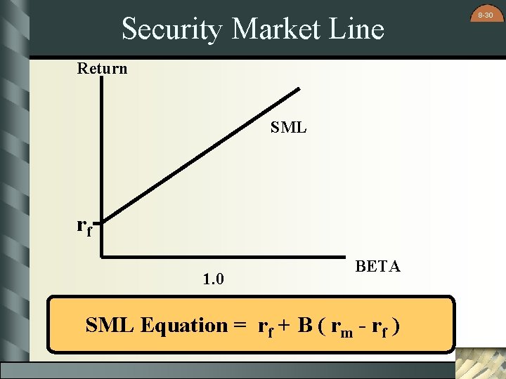
Security Market Line Return SML rf 1. 0 BETA SML Equation = rf + B ( rm - rf ) 8 -30

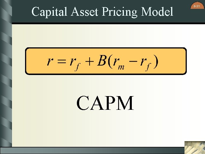
Capital Asset Pricing Model CAPM 8 -31

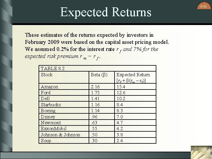
Expected Returns These estimates of the returns expected by investors in February 2009 were based on the capital asset pricing model. We assumed 0. 2% for the interest rate r f and 7% for the expected risk premium r m − r f. TABLE 8. 2 Stock Beta (β) Amazon Ford Dell Starbucks Boeing Disney Newmont Exxon. Mobil Johnson & Johnson Soup 2. 16 1. 75 1. 41 1. 16 1. 14. 96. 63. 55. 50. 30 Expected Return [rf + β(rm – rf)] 15. 4 12. 6 10. 2 8. 4 8. 3 7. 0 4. 7 4. 2 3. 8 2. 4 8 -32

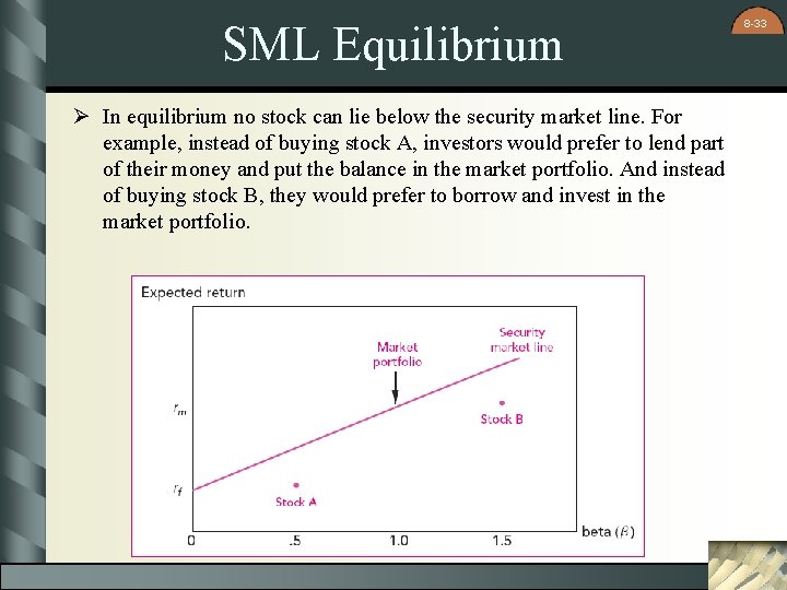
SML Equilibrium Ø In equilibrium no stock can lie below the security market line. For example, instead of buying stock A, investors would prefer to lend part of their money and put the balance in the market portfolio. And instead of buying stock B, they would prefer to borrow and invest in the market portfolio. 8 -33

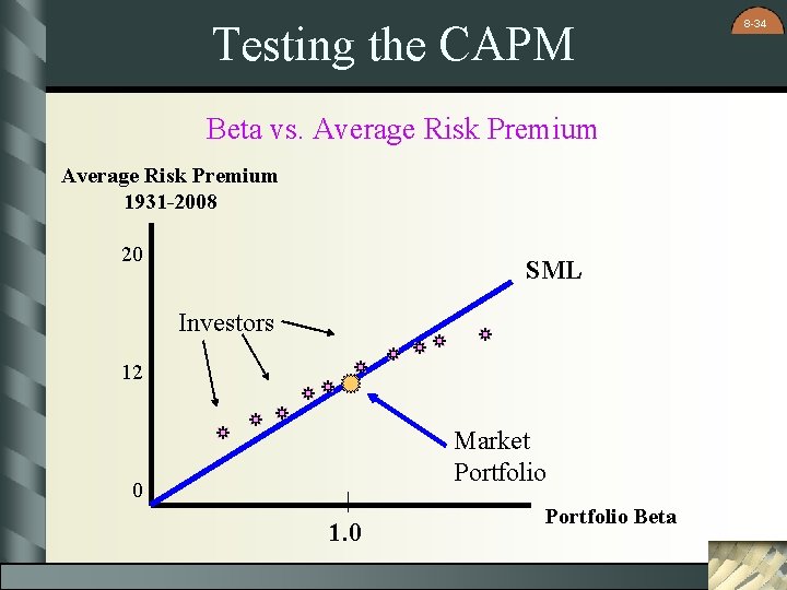
Testing the CAPM Beta vs. Average Risk Premium 1931 -2008 20 SML Investors 12 Market Portfolio 0 1. 0 Portfolio Beta 8 -34

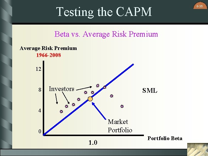
Testing the CAPM Beta vs. Average Risk Premium 1966 -2008 12 8 Investors SML 4 Market Portfolio 0 1. 0 Portfolio Beta 8 -35

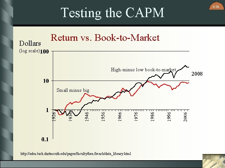
8 -36 Testing the CAPM Dollars Return vs. Book-to-Market (log scale) High-minus low book-to-market Small minus big http: //mba. tuck. dartmouth. edu/pages/faculty/ken. french/data_library. html 2008

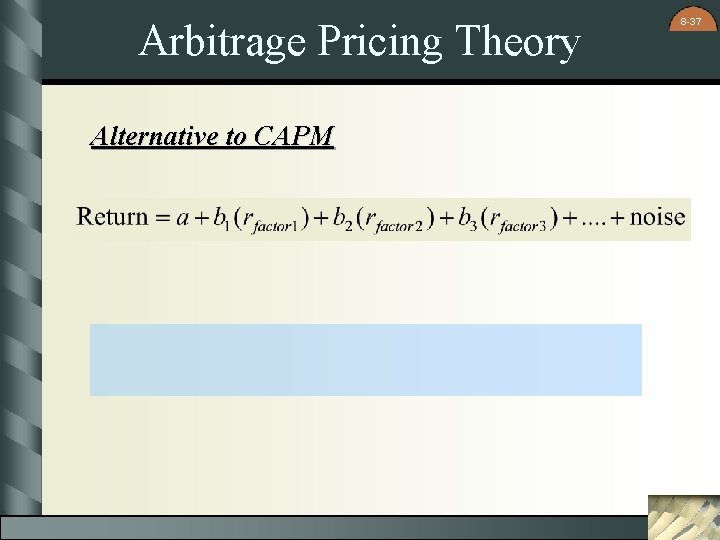
Arbitrage Pricing Theory Alternative to CAPM 8 -37

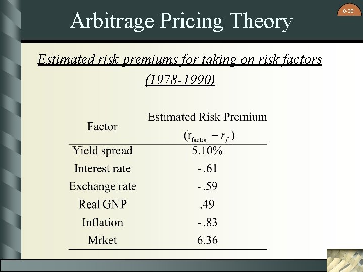
Arbitrage Pricing Theory Estimated risk premiums for taking on risk factors (1978 -1990) 8 -38

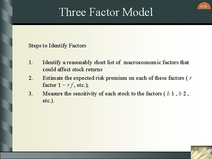
Three Factor Model Steps to Identify Factors 1. 2. 3. Identify a reasonably short list of macroeconomic factors that could affect stock returns Estimate the expected risk premium on each of these factors ( r factor 1 − r f , etc. ); Measure the sensitivity of each stock to the factors ( b 1 , b 2 , etc. ). 8 -39

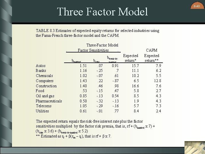
Three Factor Model TABLE 8. 3 Estimates of expected equity returns for selected industries using the Fama-French three-factor model and the CAPM. . Autos Banks Chemicals Computers Construction Food Oil and gas Pharmaceuticals Telecoms Utilities Three-Factor Model Factor Sensitivities. bmarket 1. 51 1. 16 1. 02 1. 43 1. 40. 53 0. 85 0. 50 1. 05 0. 61 bsize. 07 -. 25 -. 07. 22. 46 -. 15 -. 13 -. 32 -. 29 -. 01 bbook-tomarket 0. 91. 7. 61 -. 87. 98. 47 0. 54 -. 13 -. 16. 77 Expected return* 15. 7 11. 1 10. 2 6. 5 16. 6 5. 8 8. 5 1. 9 5. 7 8. 4 CAPM Expected return** 7. 9 6. 2 5. 5 12. 8 7. 6 2. 7 4. 3 7. 3 2. 4 The expected return equals the risk-free interest rate plus the factor sensitivities multiplied by the factor risk premia, that is, rf + (bmarket x 7) + (bsize x 3. 6) + (bbook-to-market x 5. 2) ** Estimated as rf + β(rm – rf), that is rf + β x 7. 8 -40

Web Resources Click to access web sites Internet connection required http: //finance. yahoo. com www. duke. edu/~charvey http: //mba. tuck. dartmouth. edu/pages/faculty/ken. french 8 -41