CHAPTER 8 POST OPTIMALITY ANALYSIS What is Post


")


- Slides: 18
CHAPTER 8: POST OPTIMALITY ANALYSIS
What is Post Optimality Analysis? ¨ Post Optimality Analysis – Sensitivity Analysis – What-If Analysis ¨ what happens to the optimal solution if: – THE INPUTS CHANGE: – THE CONDITIONS OF THE BUSINESS OBJECTIVE CHANGE – THE FACTORY PARAMETERS CHANGE
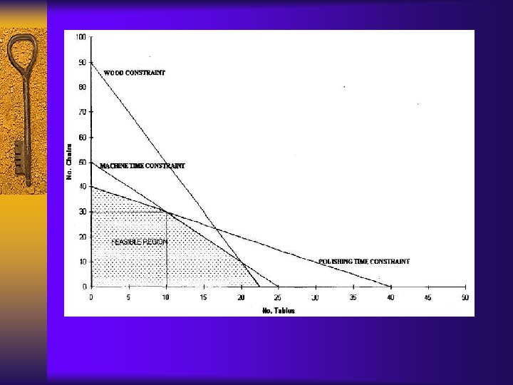
¨ Example – Let X = the number of Tables made per week, Let Y = the number of Chairs made per week, – Maximise Profit = 4 X + 3 Y Objective Function Subject to 4 X+1 Y 90 Wood 2 X+1 Y 50 Machine-Time 1 X +1 Y 40 Polishing-Time X, Y 0
Shadow Costs, Binding & Non-Binding Constraints ¨ Wood constraint – 4 X + 1 Y 90 – Optimal Solution(X, Y)=(10, 30), – the wood used 4*10+1*30=70 kilograms – 20 kilograms unused---slack value – Let RHS 90 90+1 or 90 -1 – The optimal solution does not change. – The addition or removal of one kilogram of Wood makes no difference to the optimal production plan. The Wood constraint is said to be a Non-Binding constraint.
¨ Definition of a Non-Binding Constraint – If the availability of an additional unit of a resource has no effect on the production plan, then that constraint is said to be non-binding. ¨ Definition Shadow Cost – The Shadow Cost of a resource is the additional profit generated by an additional unit of that resource. – Example: WOOD is a Non-Binding Constraint and definitionally non-binding constraints have a Shadow Cost = 0
¨ Machine-Time constraint – 2 X + 1 Y 50 – Let RHS 50 51 or 49 – The optimal solution change. – (X, Y) =(10, 30) (X, Y)=(11, 29) – Change=(1, -1)
¨ Definition Binding Constraint – If the availability of an additional unit of resource alters the optimal production plan, thereby increasing the profit, then that constraint is said to be a 'Binding Constraint'. ¨ Shadow Cost of Machine-Time – The new value of the objective function : 4*11+3*29=131 – The shadow cost of the resource Machine-Time: £ 1 ¨ Shadow Cost: A way of pricing the value of the resource
¨ The consequences of linear systems – if increasing 2 hours or decreasing 5 hours of Machine-Time became available, the new production plan would be: • (10, 30) +2*(1, -1) = (10, 30) + (2, -2) = (12, 28) • (10, 30) +(-5)*(1, -1) = (10, 30) + (-5, 5) = (5, 35) – The new profit would be : • • Old profit + 2*Shadow Cost £ 130 + 2*£ 1 = £ 132 Old profit + (-5)*Shadow Cost £ 130 + (-5)*£ 1 = £ 125
¨ Polishing-Time constraint – Polishing-Time is a binding constraint – The shadow price for Polishing-Time is £ 2 ¨ Summary RESOURCE BINDING/NON BINDING SLACK SHADOW COST WOOD NON-BINDING 20 Kgms of WOOD £ 0 MACHINE TIME BINDING 0 Hours £ 1 POLISHING TIME BINDING 0 Hours £ 2
Resource Ranging ¨ How much is it possible to increase or decrease the units of a resource whilst the shadow price is effective?
¨ Ranging for the WOOD resource Lower Limit: 70 – Existing Resource: 90 Upper Limit No upper: limit.
¨ Ranging for the MACHINE-TIME resource ¨ Lower Limit 40 Existing Resource 50 Upper Limit 56. 67
¨ The ranging for the resource POLISHING- TIME Lower Limit 30 Existing Resource 40 Upper Limit 50 ¨ Summary RESOURCE LOWER LIMIT EXISTING RESOURCE UPPER LIMIT WOOD 70 90 No upper limit. MACHINE-TIME 40 50 56. 67 POLISHING-TIME 30 40 50
Changes in the Objective Function Coefficient ¨ Introductory details – Profit = a. X + b. Y – Y=Profit/b-a/b X • Example: Profit = 4 X + 3 Y • Y = Profit/3 -4/3 X – The slope of the Machine-Time constraint • Y = 50 - 2 X – The slope of Polishing-Time constraint • Y=40 -1 X – The slope of objective function must lie between the two constraint slopes
Y = 50 - 2 X Y = Profit/b -a/b X (Y=130/3 -a/3 X) Y = 40 -1 X
– The coefficient of X can vary : 3 to 6 Slopes Machine-Time Objective -2 -a/3 Polishing-Time -1 – The coefficient of Y can vary : 2 to 4 Slopes Machine-Time -2 Objective -4/b Polishing-Time -1
The Factory Parameter Changes ¨ If the factory were to invest in different plant, new technology that had the effect of making more effective use of the input resources, how would this modify the solution to the linear programming? ¨ The practical way to see the effect this has on the linear programming is to resolve the linear programming with the new constraint