Chapter 8 Perfect Competition ECONOMICS Principles and Applications

Chapter 8 Perfect Competition ECONOMICS: Principles and Applications, 4 e HALL & LIEBERMAN, © 2008 Thomson South-Western

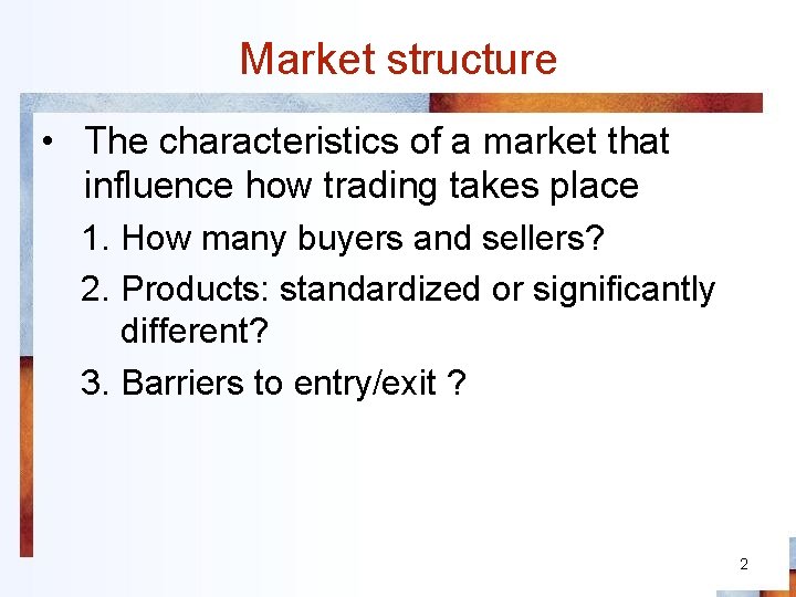
Market structure • The characteristics of a market that influence how trading takes place 1. How many buyers and sellers? 2. Products: standardized or significantly different? 3. Barriers to entry/exit ? 2

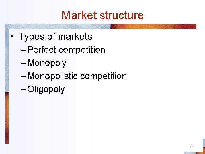
Market structure • Types of markets – Perfect competition – Monopoly – Monopolistic competition – Oligopoly 3

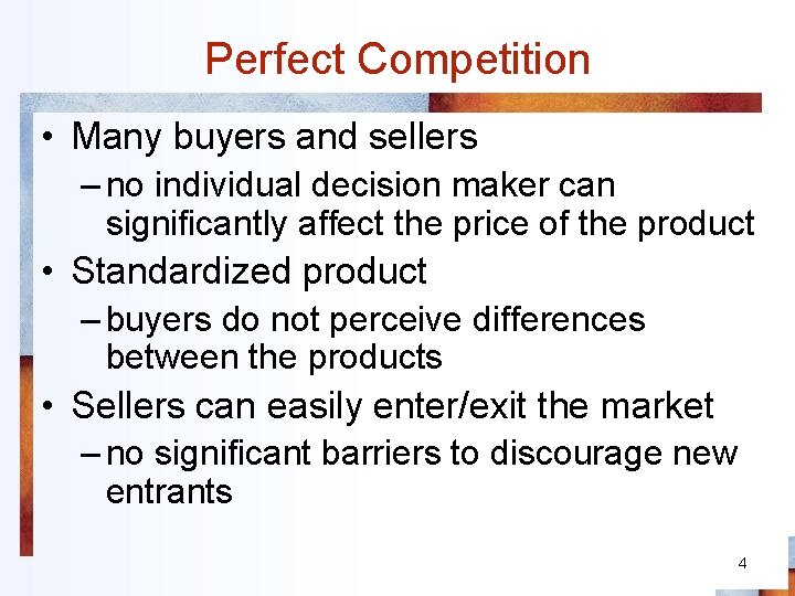
Perfect Competition • Many buyers and sellers – no individual decision maker can significantly affect the price of the product • Standardized product – buyers do not perceive differences between the products • Sellers can easily enter/exit the market – no significant barriers to discourage new entrants 4

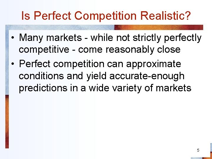
Is Perfect Competition Realistic? • Many markets - while not strictly perfectly competitive - come reasonably close • Perfect competition can approximate conditions and yield accurate-enough predictions in a wide variety of markets 5

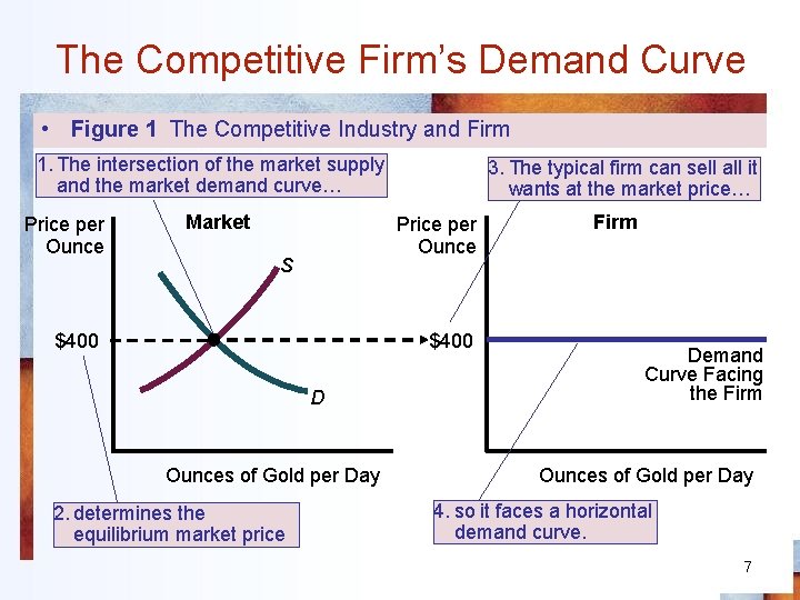
The Competitive Firm’s Demand Curve • Horizontal demand curve – perfectly elastic - at the market price • Output is standardized • Price taker – The price of its output is given • Decision – How much output to produce and sell 6

The Competitive Firm’s Demand Curve • Figure 1 The Competitive Industry and Firm 1. The intersection of the market supply and the market demand curve… Price per Ounce Market 3. The typical firm can sell all it wants at the market price… Price per Ounce S $400 D Ounces of Gold per Day 2. determines the equilibrium market price Firm Demand Curve Facing the Firm Ounces of Gold per Day 4. so it faces a horizontal demand curve. 7

Cost and Revenue Data • Marginal revenue – Is the market price • Marginal revenue curve – The demand curve facing the firm – A horizontal line at the market price 8

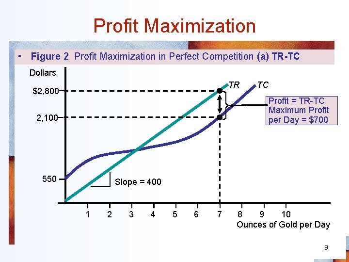
Profit Maximization • Figure 2 Profit Maximization in Perfect Competition (a) TR-TC Dollars TR $2, 800 TC Profit = TR-TC Maximum Profit per Day = $700 2, 100 550 Slope = 400 1 2 3 4 5 6 7 8 9 10 Ounces of Gold per Day 9

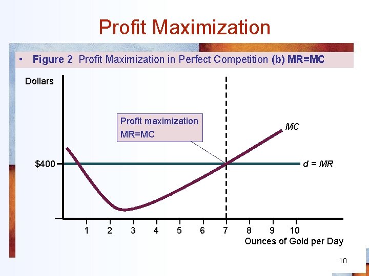
Profit Maximization • Figure 2 Profit Maximization in Perfect Competition (b) MR=MC Dollars Profit maximization MR=MC MC $400 d = MR 1 2 3 4 5 6 7 8 9 10 Ounces of Gold per Day 10

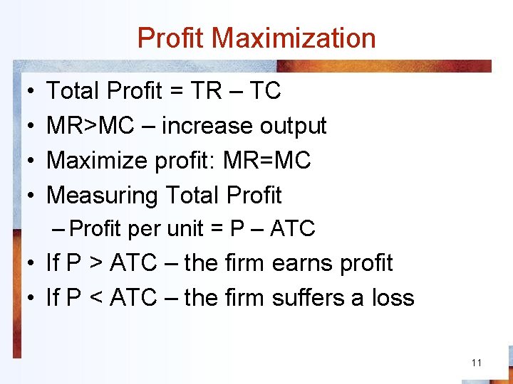
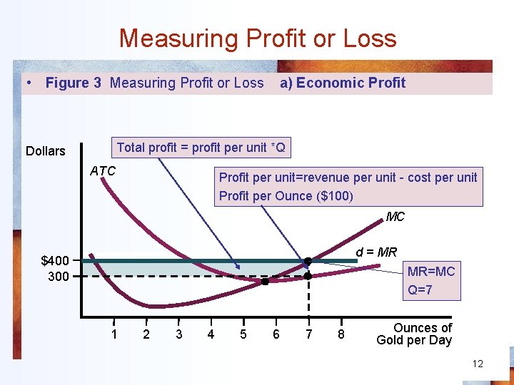
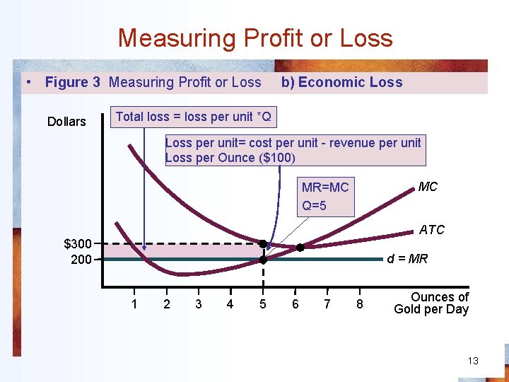
Profit Maximization • • Total Profit = TR – TC MR>MC – increase output Maximize profit: MR=MC Measuring Total Profit – Profit per unit = P – ATC • If P > ATC – the firm earns profit • If P < ATC – the firm suffers a loss 11

Measuring Profit or Loss • Figure 3 Measuring Profit or Loss a) Economic Profit Total profit = profit per unit *Q Dollars ATC Profit per unit=revenue per unit - cost per unit Profit per Ounce ($100) MC d = MR $400 300 MR=MC Q=7 1 2 3 4 5 6 7 8 Ounces of Gold per Day 12

Measuring Profit or Loss • Figure 3 Measuring Profit or Loss Dollars b) Economic Loss Total loss = loss per unit *Q Loss per unit= cost per unit - revenue per unit Loss per Ounce ($100) MC MR=MC Q=5 ATC $300 200 d = MR 1 2 3 4 5 6 7 8 Ounces of Gold per Day 13

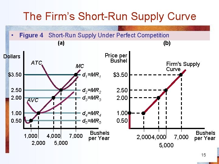
The Firm’s Short-Run Supply Curve • The firm – takes the market price as given – decides how much output to produce at that price • Profit-maximizing output level: P=MC – As price of output changes, firm will slide along its MC curve in deciding how much to produce – Exception – If the firm is suffering a loss large enough to justify shutting down 14

The Firm’s Short-Run Supply Curve • Figure 4 Short-Run Supply Under Perfect Competition (a) (b) Price per Dollars ATC Bushel MC d 1=MR 1 $3. 50 2. 00 AVC d 2=MR 2 d 3=MR 3 2. 50 2. 00 1. 00 0. 50 d 4=MR 4 d 5=MR 5 1. 00 0. 50 $3. 50 1, 000 4, 000 7, 000 2, 000 5, 000 Bushels per Year Firm's Supply Curve 2, 0004, 000 7, 000 5, 000 Bushels per Year 15

The Shutdown Price • Price at which a firm is indifferent between producing and shutting down • If P>AVC – produce • If P<AVC – shut down • Firm’s supply curve – Is its MC curve for all prices above AVC, and a vertical line at zero units for all prices below AVC. 16

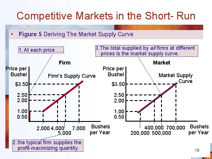
Competitive Markets in the Short- Run • Fixed number of firms in industry • Market supply curve – Quantity of output - all sellers in a market will produce at different prices – Add up the quantities of output supplied by all firms in the market at each price 17

Competitive Markets in the Short- Run • Figure 5 Deriving The Market Supply Curve 1. At each price. . . 3. The total supplied by all firms at different prices is the market supply curve. Market Firm Price per Bushel Firm's Supply Curve Price per Bushel $3. 50 2. 00 1. 00 0. 50 2, 000 4, 000 7, 000 Bushels per Year 5, 000 2. the typical firm supplies the profit-maximizing quantity. Market Supply Curve 400, 000 700, 000 Bushels per Year 200, 000 500, 000 18

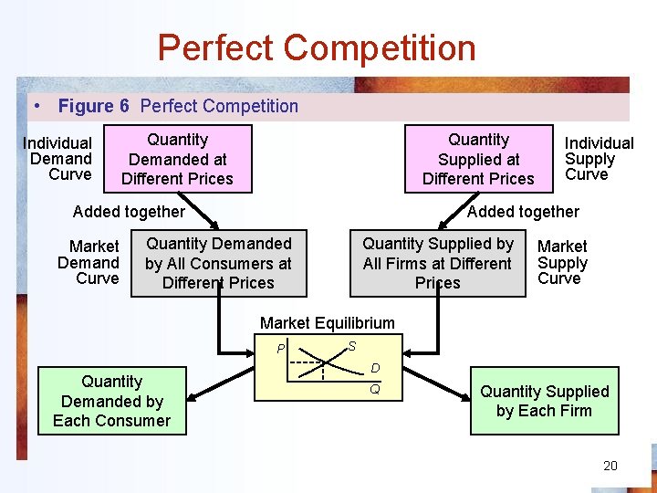
Short-Run Equilibrium • Competitive firms can earn economic profit, or suffer an economic loss • The market – sums buying and selling preferences of individual consumers and producers, and determines market price • Each buyer and seller – Takes market price as given – Is able to buy or sell the desired quantity 19

Perfect Competition • Figure 6 Perfect Competition Individual Demand Curve Quantity Demanded at Different Prices Quantity Supplied at Different Prices Added together Market Demand Curve Individual Supply Curve Added together Quantity Demanded by All Consumers at Different Prices Quantity Supplied by All Firms at Different Prices Market Supply Curve Market Equilibrium P Quantity Demanded by Each Consumer S D Q Quantity Supplied by Each Firm 20

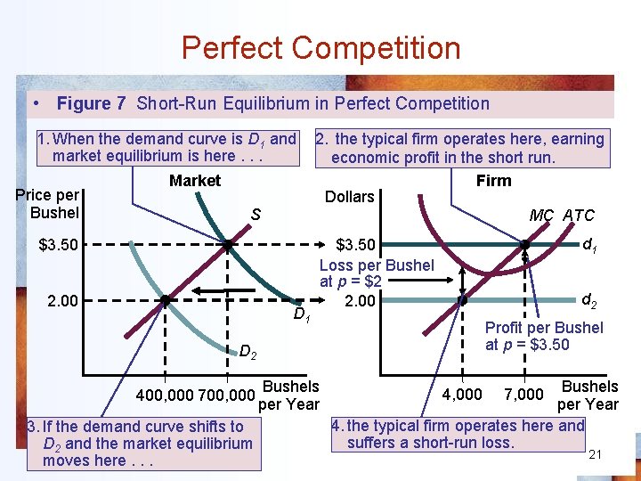
Perfect Competition • Figure 7 Short-Run Equilibrium in Perfect Competition 1. When the demand curve is D 1 and market equilibrium is here. . . Price per Bushel Market S 2. the typical firm operates here, earning economic profit in the short run. Firm Dollars MC ATC $3. 50 2. 00 D 1 d 1 $3. 50 Loss per Bushel at p = $2 2. 00 d 2 Profit per Bushel at p = $3. 50 D 2 400, 000 700, 000 3. If the demand curve shifts to D 2 and the market equilibrium moves here. . . Bushels per Year 4. the typical firm operates here and suffers a short-run loss. 4, 000 7, 000 21

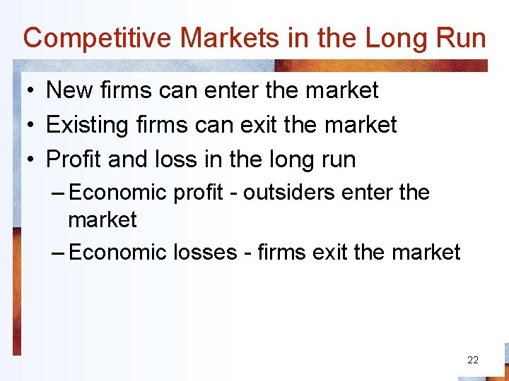
Competitive Markets in the Long Run • New firms can enter the market • Existing firms can exit the market • Profit and loss in the long run – Economic profit - outsiders enter the market – Economic losses - firms exit the market 22

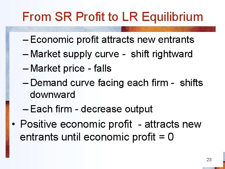
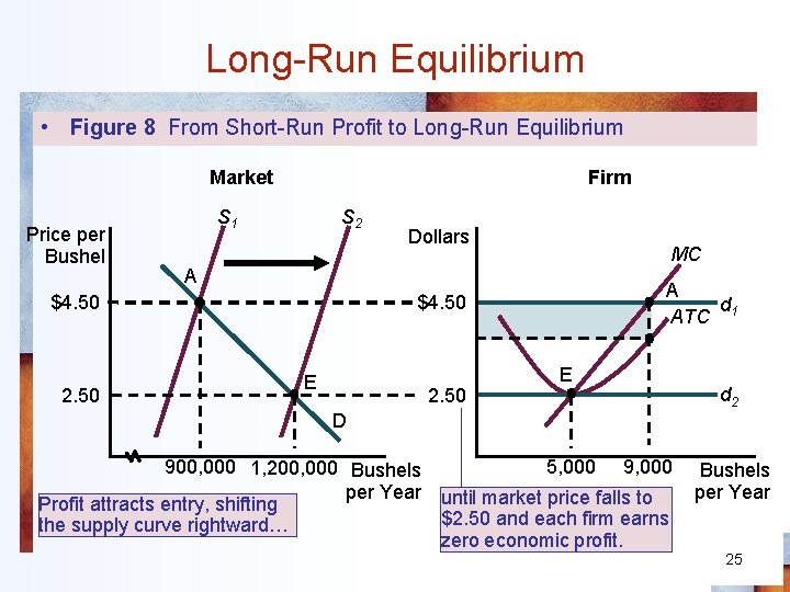
From SR Profit to LR Equilibrium – Economic profit attracts new entrants – Market supply curve - shift rightward – Market price - falls – Demand curve facing each firm - shifts downward – Each firm - decrease output • Positive economic profit - attracts new entrants until economic profit = 0 23

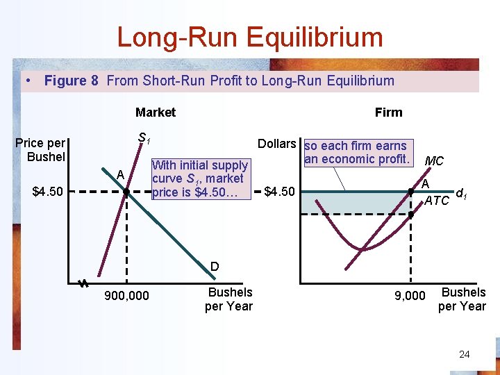
Long-Run Equilibrium • Figure 8 From Short-Run Profit to Long-Run Equilibrium Market S 1 Price per Bushel A $4. 50 Firm Dollars so each firm earns an economic profit. MC With initial supply curve S 1, market A $4. 50 price is $4. 50… d ATC 1 D 900, 000 Bushels per Year 9, 000 Bushels per Year 24

Long-Run Equilibrium • Figure 8 From Short-Run Profit to Long-Run Equilibrium Market Price per Bushel Firm S 1 S 2 MC A $4. 50 2. 50 Dollars A d ATC 1 $4. 50 E 2. 50 E d 2 D 900, 000 1, 200, 000 Bushels 5, 000 9, 000 per Year until market price falls to Profit attracts entry, shifting $2. 50 and each firm earns the supply curve rightward… zero economic profit. Bushels per Year 25

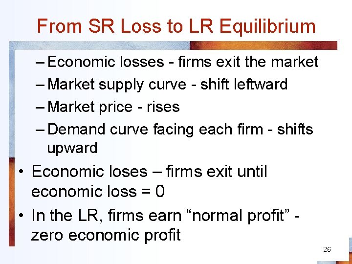
From SR Loss to LR Equilibrium – Economic losses - firms exit the market – Market supply curve - shift leftward – Market price - rises – Demand curve facing each firm - shifts upward • Economic loses – firms exit until economic loss = 0 • In the LR, firms earn “normal profit” zero economic profit 26

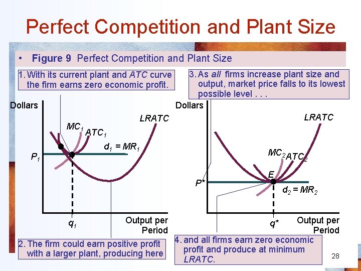
Perfect Competition and Plant Size • In LR equilibrium, every firm will select – Plant size – Output level • And – Operate at minimum point of LRATC curve 27

Perfect Competition and Plant Size • Figure 9 Perfect Competition and Plant Size 3. As all firms increase plant size and output, market price falls to its lowest possible level. . . Dollars LRATC 1. With its current plant and ATC curve the firm earns zero economic profit. Dollars MC 1 ATC 1 d 1 = MR 1 P 1 MC 2 ATC P* q 1 Output per Period 2. The firm could earn positive profit with a larger plant, producing here 2 E d 2 = MR 2 Output per Period 4. and all firms earn zero economic profit and produce at minimum 28 LRATC. q*

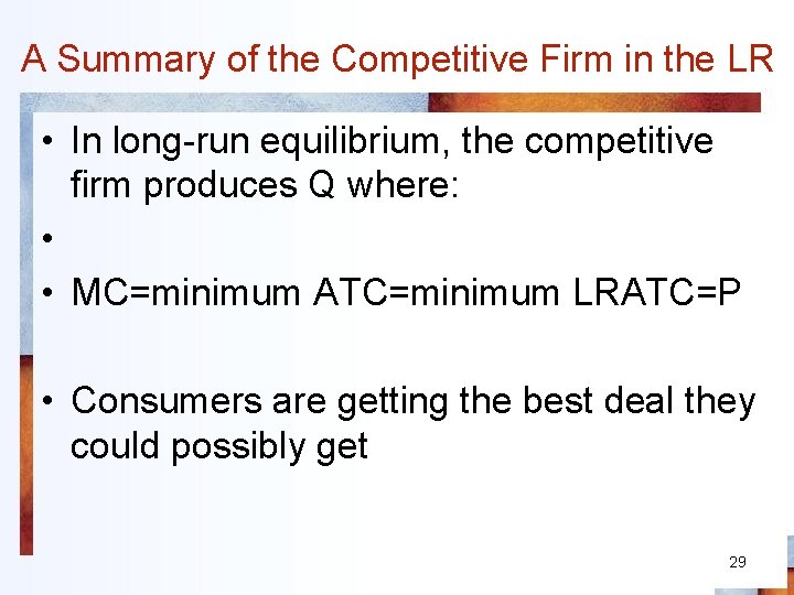
A Summary of the Competitive Firm in the LR • In long-run equilibrium, the competitive firm produces Q where: • • MC=minimum ATC=minimum LRATC=P • Consumers are getting the best deal they could possibly get 29

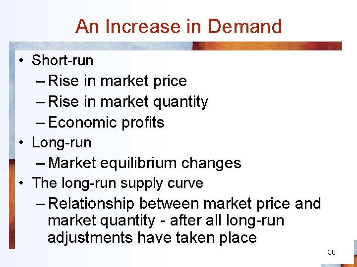
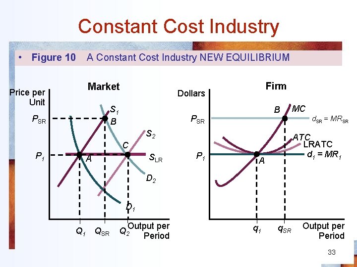
An Increase in Demand • Short-run – Rise in market price – Rise in market quantity – Economic profits • Long-run – Market equilibrium changes • The long-run supply curve – Relationship between market price and market quantity - after all long-run adjustments have taken place 30

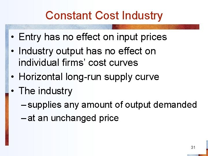
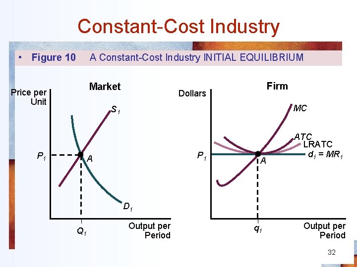
Constant Cost Industry • Entry has no effect on input prices • Industry output has no effect on individual firms’ cost curves • Horizontal long-run supply curve • The industry – supplies any amount of output demanded – at an unchanged price 31

Constant-Cost Industry • Figure 10 A Constant-Cost Industry INITIAL EQUILIBRIUM Market Price per Unit Firm Dollars MC S 1 P 1 A A ATC LRATC d 1 = MR 1 D 1 Q 1 Output per Period q 1 Output per Period 32

Constant Cost Industry • Figure 10 A Constant Cost Industry NEW EQUILIBRIUM Market Price per Unit S 1 B PSR Firm Dollars B PSR S 2 SLR A P 1 d. SR = MRSR ATC LRATC d 1 = MR 1 C P 1 MC A D 2 D 1 QSR Output per Q 2 Period q 1 q. SR Output per Period 33

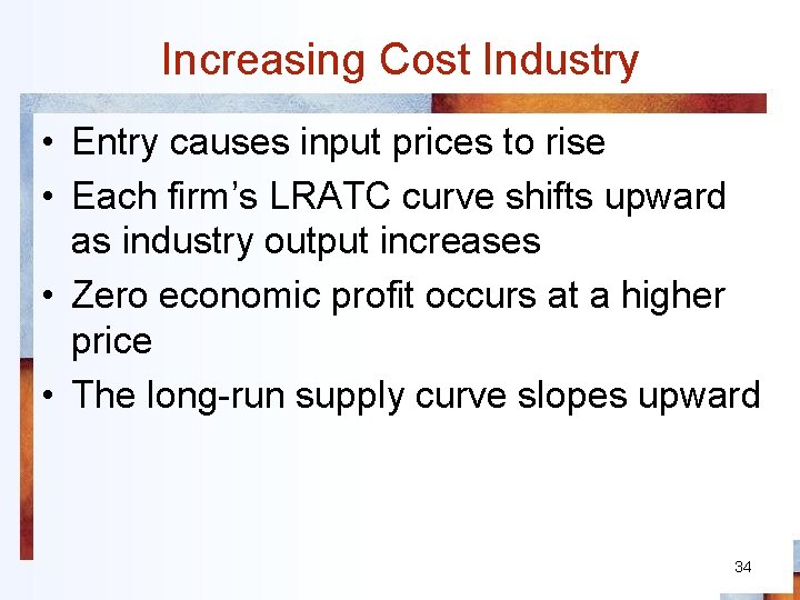
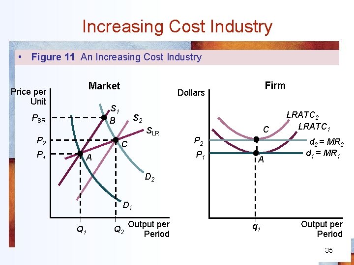
Increasing Cost Industry • Entry causes input prices to rise • Each firm’s LRATC curve shifts upward as industry output increases • Zero economic profit occurs at a higher price • The long-run supply curve slopes upward 34

Increasing Cost Industry • Figure 11 An Increasing Cost Industry Market Price per Unit S 1 B PSR S 2 SLR P 2 C P 1 Firm Dollars C P 2 P 1 A A LRATC 2 LRATC 1 d 2 = MR 2 d 1 = MR 1 D 2 D 1 Q 2 Output per Period q 1 Output per Period 35

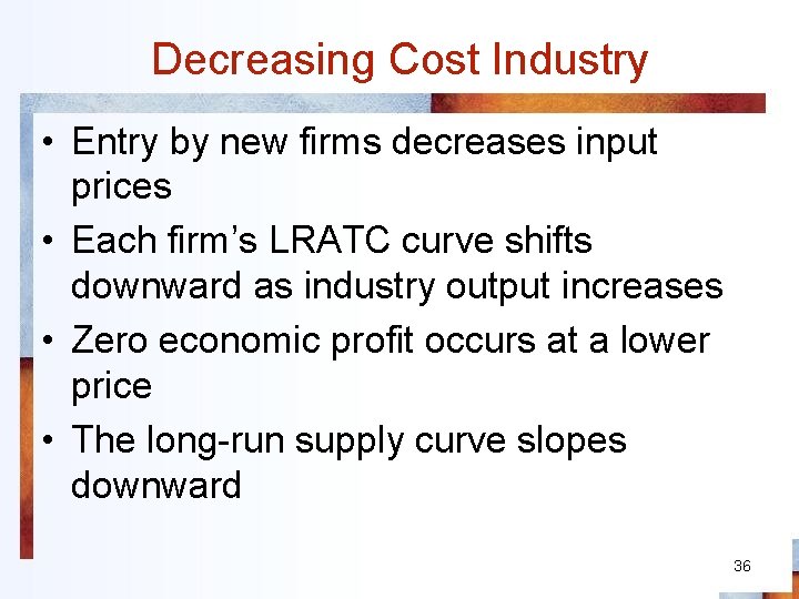
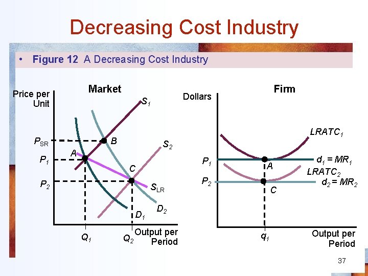
Decreasing Cost Industry • Entry by new firms decreases input prices • Each firm’s LRATC curve shifts downward as industry output increases • Zero economic profit occurs at a lower price • The long-run supply curve slopes downward 36

Decreasing Cost Industry • Figure 12 A Decreasing Cost Industry Market Price per Unit S 1 PSR P 1 LRATC 1 B S 2 A P 1 C P 2 SLR D 1 Q 1 Firm Dollars Q 2 A P 2 C d 1 = MR 1 LRATC 2 d 2 = MR 2 D 2 Output per Period q 1 Output per Period 37

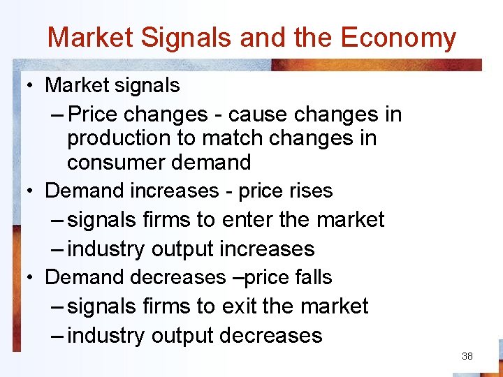
Market Signals and the Economy • Market signals – Price changes - cause changes in production to match changes in consumer demand • Demand increases - price rises – signals firms to enter the market – industry output increases • Demand decreases –price falls – signals firms to exit the market – industry output decreases 38

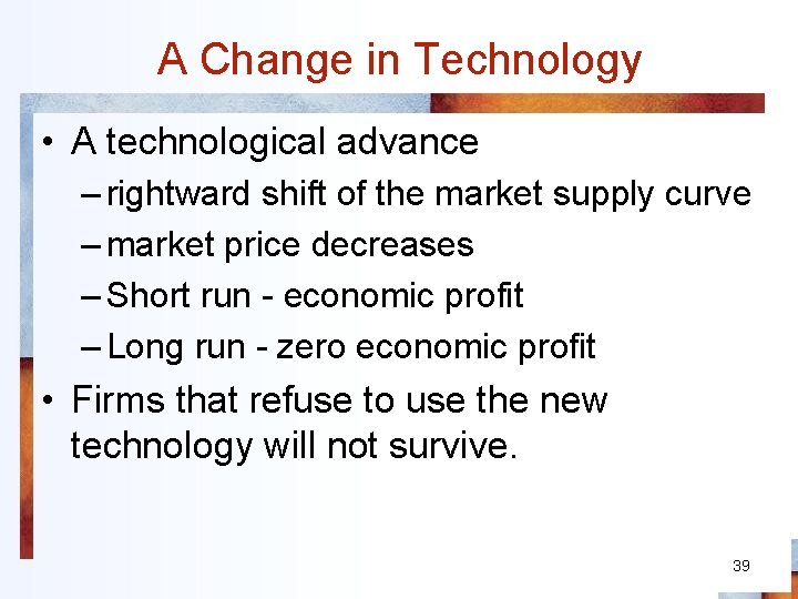
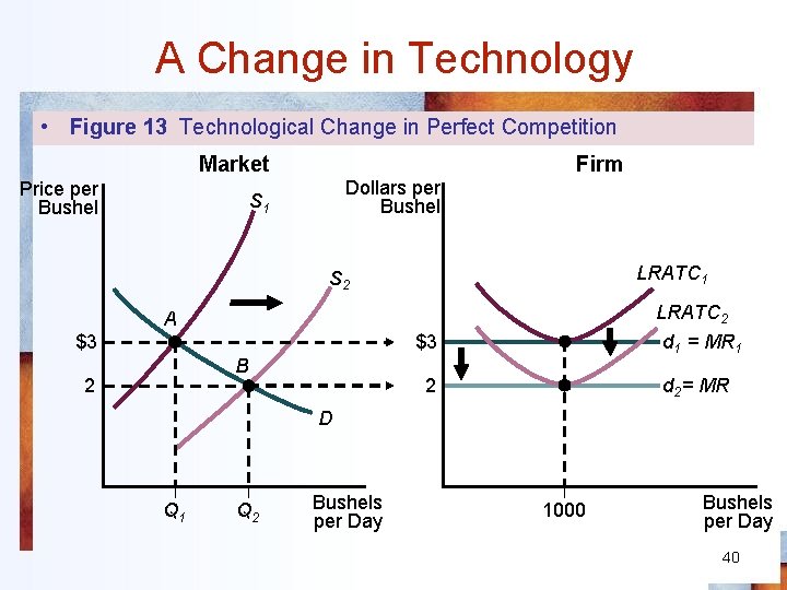
A Change in Technology • A technological advance – rightward shift of the market supply curve – market price decreases – Short run - economic profit – Long run - zero economic profit • Firms that refuse to use the new technology will not survive. 39

A Change in Technology • Figure 13 Technological Change in Perfect Competition Firm Market Price per Bushel Dollars per Bushel S 1 LRATC 1 S 2 $3 LRATC 2 d 1 = MR 1 2 d 2= MR A $3 B 2 D Q 1 Q 2 Bushels per Day 1000 Bushels per Day 40

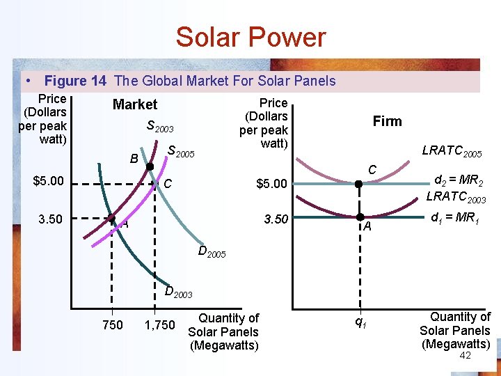
Solar Power: Increasing Cost Industry • Generating electricity from solar panels – costs more than twice as much as generating the same energy from fossil fuels • With government help – by 2006, Germany became the world’s largest producer of solar energy • The growth slowed dramatically in early 2006 – even though the subsidies and incentives remained 41 • The solar panel industry - increasing cost

Solar Power • Figure 14 The Global Market For Solar Panels Price (Dollars per peak watt) S 2003 B $5. 00 3. 50 Price (Dollars per peak watt) Market S 2005 C Firm LRATC 2005 C $5. 00 3. 50 A A d 2 = MR 2 LRATC 2003 d 1 = MR 1 D 2005 D 2003 750 1, 750 Quantity of Solar Panels (Megawatts) q 1 Quantity of Solar Panels (Megawatts) 42

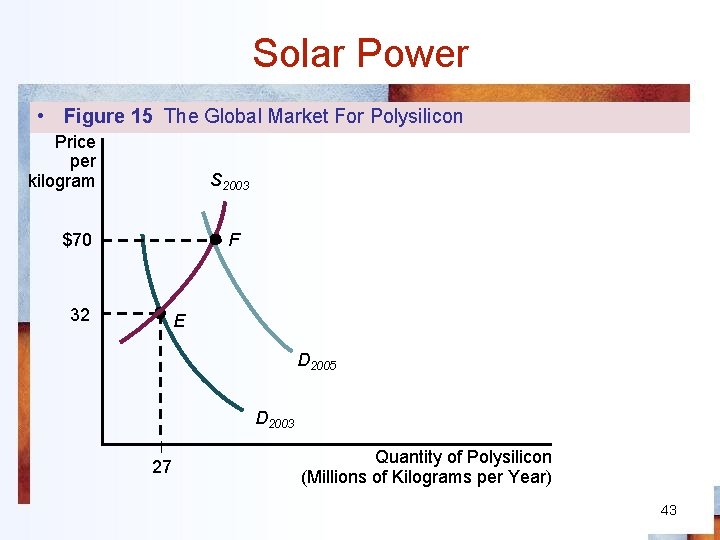
Solar Power • Figure 15 The Global Market For Polysilicon Price per kilogram S 2003 $70 F 32 E D 2005 D 2003 27 Quantity of Polysilicon (Millions of Kilograms per Year) 43