Chapter 8 Perfect competition and pure monopoly David

Chapter 8 Perfect competition and pure monopoly David Begg, Stanley Fischer and Rudiger Dornbusch, Economics, 9 th Edition, Mc. Graw-Hill, 2008 Power. Point presentation by Alex Tackie and Damian Ward ©The Mc. Graw-Hill Companies, 2008

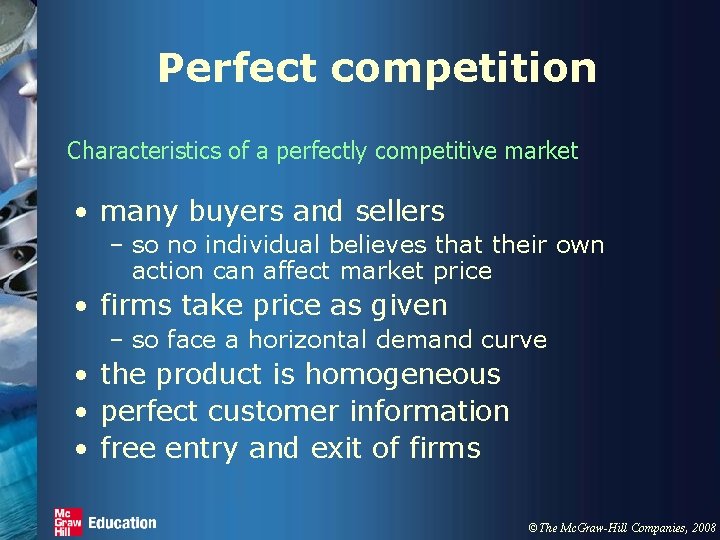
Perfect competition Characteristics of a perfectly competitive market • many buyers and sellers – so no individual believes that their own action can affect market price • firms take price as given – so face a horizontal demand curve • the product is homogeneous • perfect customer information • free entry and exit of firms ©The Mc. Graw-Hill Companies, 2008

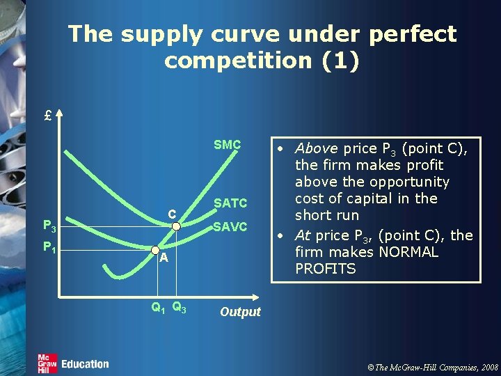
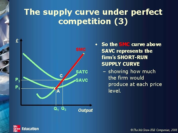
The supply curve under perfect competition (1) £ SMC P 3 P 1 C SATC SAVC A Q 1 Q 3 • Above price P 3 (point C), the firm makes profit above the opportunity cost of capital in the short run • At price P 3, (point C), the firm makes NORMAL PROFITS Output ©The Mc. Graw-Hill Companies, 2008

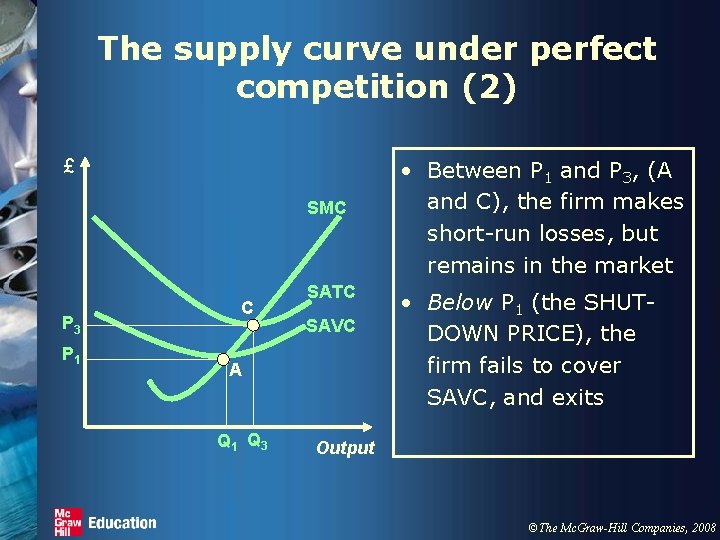
The supply curve under perfect competition (2) £ SMC P 3 P 1 C SATC SAVC A Q 1 Q 3 • Between P 1 and P 3, (A and C), the firm makes short-run losses, but remains in the market • Below P 1 (the SHUTDOWN PRICE), the firm fails to cover SAVC, and exits Output ©The Mc. Graw-Hill Companies, 2008

The supply curve under perfect competition (3) £ SMC P 3 P 1 C SATC SAVC A Q 1 Q 3 • So the SMC curve above SAVC represents the firm’s SHORT-RUN SUPPLY CURVE – showing how much the firm would produce at each price level. Output ©The Mc. Graw-Hill Companies, 2008

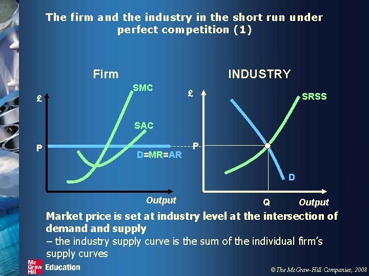
The firm and the industry in the short run under perfect competition (1) Firm INDUSTRY SMC £ £ SRSS SAC P D=MR=AR P D Output Q Output Market price is set at industry level at the intersection of demand supply – the industry supply curve is the sum of the individual firm’s supply curves ©The Mc. Graw-Hill Companies, 2008

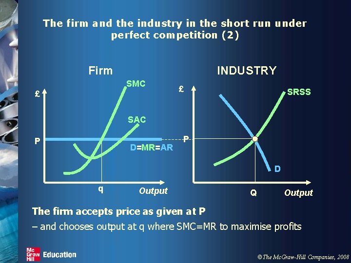
The firm and the industry in the short run under perfect competition (2) Firm INDUSTRY SMC £ £ SRSS SAC P D=MR=AR P D q Output Q Output The firm accepts price as given at P – and chooses output at q where SMC=MR to maximise profits ©The Mc. Graw-Hill Companies, 2008

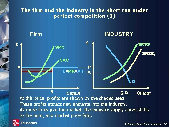
The firm and the industry in the short run under perfect competition (3) Firm INDUSTRY £ £ SMC SRSS 1 SAC P D=MR=AR P 1 P D q Output Q Q 1 Output At this price, profits are shown by the shaded area. These profits attract new entrants into the industry. As more firms join the market, the industry supply curve shifts to the right, and market price falls. ©The Mc. Graw-Hill Companies, 2008

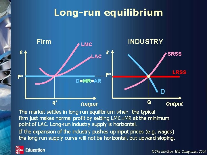
Long-run equilibrium Firm INDUSTRY LMC £ LAC £ SRSS LRSS P* P* D=MR=AR D Q Output The market settles in long-run equilibrium when the typical firm just makes normal profit by setting LMC=MR at the minimum point of LAC. Long-run industry supply is horizontal. If the expansion of the industry pushes up input prices (e. g. wages) the long-run supply curve will not be horizontal, but upward-sloping. q* ©The Mc. Graw-Hill Companies, 2008

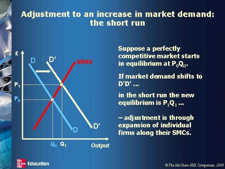
Adjustment to an increase in market demand: the short run £ D D' Suppose a perfectly competitive market starts in equilibrium at P 0 Q 0. SRSS If market demand shifts to D'D'. . . P 1 in the short run the new equilibrium is P 1 Q 1. . . P 0 D Q 0 Q 1 D' – adjustment is through expansion of individual firms along their SMCs. Output ©The Mc. Graw-Hill Companies, 2008

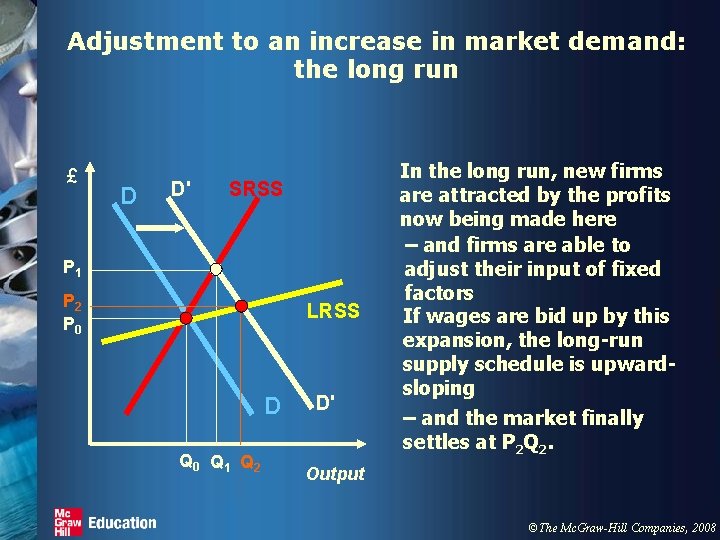
Adjustment to an increase in market demand: the long run £ D D' SRSS P 1 P 2 P 0 LRSS D Q 0 Q 1 Q 2 D' In the long run, new firms are attracted by the profits now being made here – and firms are able to adjust their input of fixed factors If wages are bid up by this expansion, the long-run supply schedule is upwardsloping – and the market finally settles at P 2 Q 2. Output ©The Mc. Graw-Hill Companies, 2008

Monopoly • A monopolist: – is the sole supplier of an industry’s product • and the only potential supplier – is protected by some form of barrier to entry – faces the market demand curve directly – Unlike under perfect competition, MR is always below AR. ©The Mc. Graw-Hill Companies, 2008

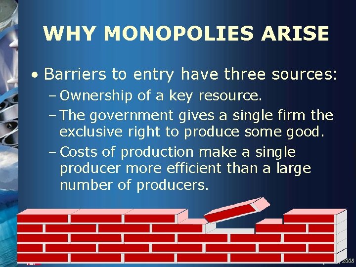
WHY MONOPOLIES ARISE • Barriers to entry have three sources: – Ownership of a key resource. – The government gives a single firm the exclusive right to produce some good. – Costs of production make a single producer more efficient than a large number of producers. ©The Mc. Graw-Hill Companies, 2008

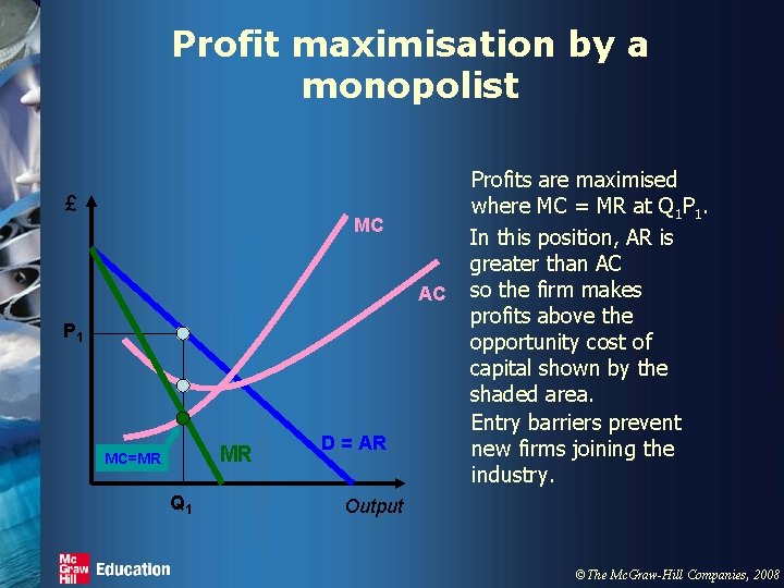
Profit maximisation by a monopolist £ MC AC P 1 MR MC=MR Q 1 D = AR Profits are maximised where MC = MR at Q 1 P 1. In this position, AR is greater than AC so the firm makes profits above the opportunity cost of capital shown by the shaded area. Entry barriers prevent new firms joining the industry. Output ©The Mc. Graw-Hill Companies, 2008

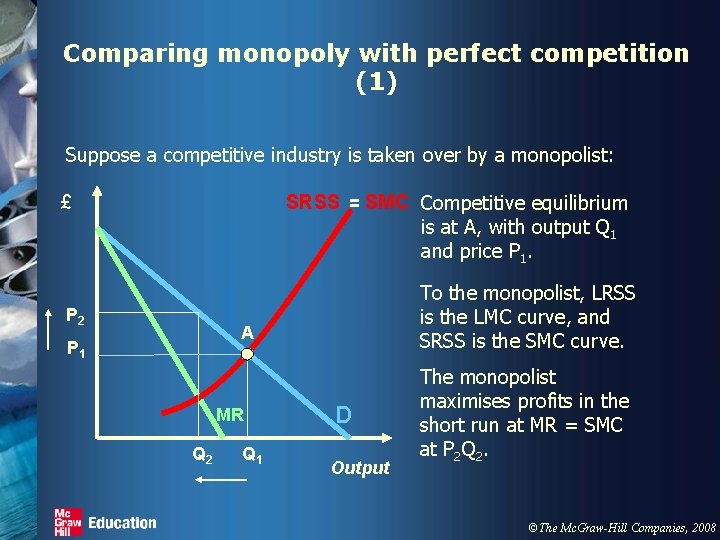
Comparing monopoly with perfect competition (1) Suppose a competitive industry is taken over by a monopolist: SRSS = SMC Competitive equilibrium is at A, with output Q 1 and price P 1. £ P 2 To the monopolist, LRSS is the LMC curve, and SRSS is the SMC curve. A P 1 MR Q 2 Q 1 D Output The monopolist maximises profits in the short run at MR = SMC at P 2 Q 2. ©The Mc. Graw-Hill Companies, 2008

Comparing monopoly with perfect competition (2) • So we see that monopoly compared with perfect competition implies: – higher price – lower output • Does the consumer always lose from monopoly? – Among other things, this depends on whether the monopolist faces the same cost structure – there may be the possibility of economies of scale. ©The Mc. Graw-Hill Companies, 2008

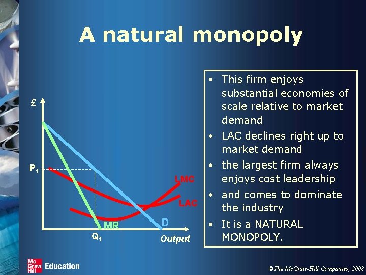
A natural monopoly • This firm enjoys substantial economies of scale relative to market demand £ • LAC declines right up to market demand P 1 LMC LAC Q 1 MR D Output • the largest firm always enjoys cost leadership • and comes to dominate the industry • It is a NATURAL MONOPOLY. ©The Mc. Graw-Hill Companies, 2008

Discriminating monopoly • Suppose a monopolist supplies two separate groups of customers – with differing elasticities of demand – e. g. business travellers may be less sensitive to air fare levels than tourists. • The monopolist may increase profits by charging higher prices to the businessmen than to tourists. • Discrimination is more likely to be possible for goods that cannot be resold – e. g. dental treatment. ©The Mc. Graw-Hill Companies, 2008

Monopoly and Perfect Competition (Summary) • Monopoly versus Competition – Monopoly • Is the sole producer • Faces a downward-sloping demand curve • Is a price maker • Make supernormal profits. P>MC – Competitive Firm • Is one of many producers • Faces a horizontal demand curve • Is a price taker • Make zero (normal) profits. P=MC ©The Mc. Graw-Hill Companies, 2008