Chapter 8 Making Capital Investment Decisions Key Concepts

Chapter 8 Making Capital Investment Decisions

Key Concepts and Skills � � � Determine the relevant cash flows for various types of capital investments Compute depreciation expense for tax purposes Incorporate inflation into capital budgeting Employ the various methods for computing operating cash flow Apply the Equivalent Annual Cost approach

Incremental Cash Flows Cash flows matter—not accounting earnings. � Incremental cash flows matter. � ◦ Sunk costs don’t matter. ◦ Opportunity costs matter. Side effects like cannibalism and erosion matter. � Taxes matter: we want incremental aftertax cash flows. � Inflation matters. � STAND ALONE PRINCIPLE – view the Project as a mini-firm.

Cash Flow: The Basis of Capital Budgeting Decisions � When performing capital budgeting analysis: ◦ Always base calculations on cash flow, not income �Earnings ≠ Cash �Need cash for capital spending �Need cash for rewarding shareholders �Therefore, capital expenditure analysis must be based on cash � Much of the work in evaluating a project lies in converting accounting income to cash flow (e. g. , Depreciation)

Incremental Cash Flows � Remember: Incremental cash flows arise as a consequence of selecting a project � Sunk costs are not relevant ◦ Just because “we have come this far” does not mean that we should continue to throw good money after bad. � Opportunity costs do matter. Just because a project has a positive NPV, that does not mean that it should also have automatic acceptance. Specifically, if another project with a higher NPV would have to be passed up, then we should not proceed.

Sunk Costs vs. Opportunity Costs � Last year, you purchased a plot of land for $2. 5 million. � Currently, its market value is $2. 0 million. � You are considering placing a new retail outlet on this land. How should the land cost be evaluated for purposes of projecting the cash flows that will become part of the NPV analysis?

Incremental Cash Flows � Side effects matter. ◦ Erosion and cannibalism are both bad things. If our new product causes existing customers to demand less of current products, we need to recognize that. � For example, erosion: cash flow transferred from existing operations to the new project. Starbucks introduction of “Via” Apple offering an i. Pad 3/4 or Mini-i. Pad. ◦ If, however, synergies result that create increased demand of existing products, we also need to recognize that.

Incremental Cash Flows � Allocations ◦ Overhead may be allocated to the new project ◦ Allocations are only relevant if the project increases or decreases the cash outlay of the entire firm � Salvage Value ◦ Don’t forget to treat salvage value (after tax, of course) as a cash inflow at the end of the project � Changes in Net Working Capital ◦ Many projects require an increase in NWC (inventory, receivables, and other current assets) when initiated; this is a cash outlay at the beginning of the project ◦ Don’t forget: To reduce NWC at the end of a project requiring increased NWC; this is a cash inflow at the end of the project

Taxes and capital budgeting – Depreciation and Salvage value � Accountants charge depreciation to spread a fixed asset’s costs over time to match its benefits � Capital budgeting analysis focuses on cash inflows and outflows when they occur � Non-cash expenses affect cash flow through their impact on taxes ◦ Compute after-tax net income and add depreciation back ◦ Ignore depreciation expense but add back its tax savings � For capital budgeting analysis, it is the depreciation method for tax purposes that matters

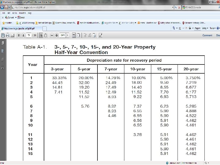
How much depreciation can be taken? � Modified Accelerated Cost Recovery System (ACRS): 1986 Tax Reform Act allows firms to "front-load" depreciation charges. � Modified ACRS Property Classes: ◦ 3 year (short lived equipment, including research) ◦ 5 year (autos, computers, etc. ) ◦ 7 year (most industrial equipment)

Salvage Value and Taxes on Sale of Fixed Assets Tax = [Selling price - Book value]x[Tax rate] Example 1. Selling price = $100, 000, Book value = $80, 000. Tax = [100, 000 - 80, 000][. 40] = $8, 000 Total Cashflow from sale of asset: $100, 000$8, 000=$92, 000 Example 2. Selling price = $50, 000, Book value = $80, 000. Tax = [50, 000 - 80, 000][. 40] = -$12, 000 Total Cashflow from sale of asset: $50, 000+$12, 000=$62, 000

Estimating Net Cash Flows – also known as Free Cash Flows or Cash Flows from Assets � Operating Cash Flow ◦ Recall that: OCF = EBIT – Taxes + Depreciation � Net Capital Spending or Capital Expenditures ◦ Don’t forget salvage value (after tax, of course). � Changes in Net Working Capital ◦ Recall that when the project winds down, we enjoy a return of net working capital.

Alternative Methods for Computing OCF � Bottom-Up Approach ◦ Works only when there is no interest expense ◦ OCF = NI + depreciation � Top-Down Approach ◦ OCF = Sales – Costs – Taxes ◦ Don’t subtract non-cash deductions � Tax Shield Approach ◦ OCF = (Sales – Costs)(1 – T) + Depreciation*T ◦ (R-E-D) *(1 -t) + D = OCF

Interest Expense � Later chapters will deal with the impact that the amount of debt that a firm has in its capital structure has on firm value. � For now, it’s enough to assume that the firm’s level of debt (and, hence, interest expense) is independent of the project at hand.

Inflation and Capital Budgeting � � Inflation is an important fact of economic life and must be considered in capital budgeting. Consider the relationship between interest rates and inflation, often referred to as the Fisher equation: (1 + Nominal Rate) = (1 + Real Rate) × (1 + Inflation Rate) � � � For low rates of inflation, this is often approximated: Real Rate Nominal Rate – Inflation Rate While the nominal rate in the U. S. has fluctuated with inflation, the real rate has generally exhibited far less variance than the nominal rate. In capital budgeting, one must compare real cash flows discounted at real rates or nominal cash flows discounted at nominal rates.

The Baldwin Company – Section 8. 2 of RWJJ q q q Costs of test marketing (already spent): $250, 000 Current market value of proposed factory site (which we own): $150, 000 Cost of bowling ball machine: $100, 000 (depreciated according to MACRS 5 -year) Increase in net working capital: $10, 000 Production (in units) by year during 5 -year life of the machine: 5, 000, 8, 000, 12, 000, 10, 000, 6, 000

The Baldwin Company q Price during first year is $20; price increases 2% per year thereafter. q Production costs during first year are $10 per unit and increase 10% per year thereafter. q Annual inflation rate: 5% q Working Capital: initial $10, 000 changes with sales

The Baldwin Company ($ thousands) (All cash flows occur at the end of the year. ) Year 0 Year 1 Year 2 Year 3 Year 4 Investments: (1) Bowling ball machine – 100. 00 (2) Accumulated 20. 00 52. 00 71. 20 depreciation (3) Adjusted basis of 80. 00 48. 00 28. 80 machine after depreciation (EOY) (4) Opportunity cost – 150. 00 (warehouse) (5) Net working capital 10. 00 16. 32 24. 97 (6) Change in NWC – 10. 00 – 6. 32 – 8. 65 (7) Total cash flow of – 260. 00 – 6. 32 – 8. 65 investment [(1) + (4) + (6)] Year 5 82. 72 21. 76* 94. 24 17. 28 5. 76 150. 00 21. 22 3. 75 0 21. 22 192. 98

The Baldwin Company After-Tax salvage Value with Mkt Value $30, 000 and Cap gain of (30 -5. 76=24. 24) Year 0 Year 1 Year 2 Year 3 Year 4 Year 5 52. 00 71. 20 82. 72 21. 76* 94. 24 48. 00 28. 80 17. 28 5. 76 Investments: (1) Bowling ball machine – 100. 00 (2) Accumulated 20. 00 depreciation (3) Adjusted basis of 80. 00 machine after depreciation (end of year) (4) Opportunity cost – 150. 00 (warehouse) (5) Net working capital 10. 00 (end of year) (6) Change in NWC – 10. 00 (7) Total cash flow of – 260. 00 investment [(1) + (4) + (6)] 150. 00 16. 32 – 6. 32 24. 97 21. 22 – 8. 65 3. 75 0 21. 22 192. 98 At the end of the project, the warehouse is unencumbered, so we can sell it if we want to.

The Baldwin Company Income: (8) Sales Revenues Year 0 Year 1 Year 2 Year 3 Year 4 Year 5 100. 00 163. 20 249. 72 212. 20 129. 90 Recall that production (in units) by year during the 5 -year life of the machine is given by: (5, 000, 8, 000, 12, 000, 10, 000, 6, 000). Price during the first year is $20 and increases 2% per year thereafter. Sales revenue in year 3 = 12, 000×[$20×(1. 02)2]=12, 000×$20. 81=$249, 720.

The Baldwin Company Income: (8) Sales Revenues (9) Operating costs Year 0 Year 1 Year 2 Year 3 Year 4 Year 5 100. 00 50. 00 163. 20 88. 00 249. 72 145. 20 212. 20 129. 90 133. 10 87. 84 Again, production (in units) by year during 5 -year life of the machine is given by: (5, 000, 8, 000, 12, 000, 10, 000, 6, 000). Production costs during the first year (per unit) are $10, and they increase 10% per year thereafter. Production costs in year 2 = 8, 000×[$10×(1. 10)1] = $88, 000

The Baldwin Company Income: (8) Sales Revenues (9) Operating costs (10) Depreciation Year 0 Year 1 Year 2 Year 3 100. 00 50. 00 20. 00 163. 20 88. 00 32. 00 249. 72 212. 20 129. 90 145. 20 133. 10 87. 84 19. 20 11. 52 Depreciation is calculated using the Accelerated Cost Recovery System (shown at right). Our cost basis is $100, 000. Depreciation charge in year 4 = $100, 000×(. 1152) = $11, 520. Year 1 2 3 4 5 6 Total Year 4 ACRS % 20. 00% 32. 00% 19. 20% 11. 52% 5. 76% 100. 00% Year 5

The Baldwin Company Year 0 Year 1 Year 2 Year 3 Year 4 Income: (8) Sales Revenues (9) Operating costs (10) Depreciation (11) Income before taxes [(8) – (9) - (10) (12) Tax at 34 percent (13) Net Income Add back depreciation (13) OCF Year 5 100. 00 163. 20 249. 72 212. 20 129. 90 50. 00 88. 00 145. 20 133. 10 87. 84 20. 00 32. 00 19. 20 11. 52 30. 00 43. 20 85. 32 67. 58 30. 54 10. 20 19. 80 20. 00 14. 69 28. 51 32. 00 29. 01 56. 31 19. 20 22. 98 44. 60 11. 52 10. 38 20. 16 11. 52 39. 80 60. 51 75. 51 56. 12 31. 68

Incremental After Tax Cash Flows Year 0 Year 1 Year 2 Year 3 Year 4 Year 5 (1) Sales Revenues (2) Operating costs (3) Taxes $100. 00 $163. 20 $249. 72 $212. 20 $129. 90 -50. 00 -88. 00 -145. 20 133. 10 -87. 84 -10. 20 -14. 69 -29. 01 -22. 98 -10. 38 (4) OCF (1) – (2) – (3) (5) Total CF of Investment (6) IATCF [(4) + (5)] 39. 80 60. 51 75. 51 56. 12 31. 68 – 260. – 6. 32 – 8. 65 3. 75 192. 98 – 260. 39. 80 54. 19 66. 86 59. 87 224. 66

Investments of Unequal Lives � There are times when blunt application of the NPV rule can lead to the wrong decision. Consider a factory that must have an air cleaner that is mandated by law. There are two choices: ◦ The “Cadillac cleaner” costs $4, 000 today, has annual operating costs of $100, and lasts 10 years. ◦ The “Cheapskate cleaner” costs $1, 000 today, has annual operating costs of $500, and lasts 5 years. � Assuming a 10% discount rate, which one should we choose?

NPV Calculation � NPVCad = -4000 + -100*A 0. 1, 10 ◦ A 0. 1, 10= 6. 1446 ◦ NPVCad = - 4614. 46 � NPVCheap = -1000 + -500*A 0. 1, 5 ◦ A 0. 1, 5= 3. 7908 ◦ NPVCheap = -2895. 39 At first glance, the Cheapskate cleaner has a higher NPV.

Investments of Unequal Lives Cadillac Air Cleaner CF 0 – 4, 000 Cheapskate Air Cleaner CF 0 – 1, 000 CF 1 – 100 CF 1 – 500 F 1 10 F 1 5 I 10 NPV – 4, 614. 46 NPV – 2, 895. 39 At first glance, the Cheapskate cleaner has a higher NPV.

Investments of Unequal Lives But the Cadillac lasts twice as long! � Replacement Chain � ◦ Repeat projects until they begin and end at the same time. ◦ Compute NPV for the “repeated projects. ” � The Equivalent Annual Cost Method (EAC) ◦ Applicable to a much more robust set of circumstances than the replacement chain ◦ The EAC is the value of the level payment annuity that has the same PV as our original set of cash flows. � I HIGHLY RECOMMEND YOU USE THE EAC METHOD!

EAC Calculation � EACCad = 4614. 46/A 0. 1, 10 ◦ A 0. 1, 10= 6. 1446 ◦ EAC = 750. 98 � EACCheap = 2895. 39/A 0. 1, 5 ◦ A 0. 1, 5= 3. 7908 ◦ EAC = 763. 79 � We should purchase the Cadillac because it has lower annual costs.

Equivalent Annual Cost (EAC) � EAC is the annual annuity payment implied by a project’s NPV � In other words: ◦ if the present value of an annuity is set equal to the project NPV ◦ and an annual payment is computed ◦ using the same term and rate as the NPV; then, ◦ the payment is the EAC � The EAC for the Cadillac filter is $750. 98 � The EAC for the Cheapskate filter is $763. 98 � In general, select the EAC with the lower cost. This suggests a decision to reject the Cheapskate filter which had the more attractive raw NPV

Cadillac EAC with a Calculator Net Present Value Equivalent Annual Cost N 10 – 100 I/Y 10 F 1 10 PV – 4, 614. 46 I 10 PMT 750. 98 CF 0 – 4, 000 CF 1 NPV – 4, 614. 46 FV

Cheapskate EAC with a Calculator Net Present Value Equivalent Annual Cost N 5 – 500 I/Y 10 F 1 5 PV -2, 895. 39 I 10 PMT 763. 80 CF 0 – 1, 000 CF 1 NPV – 2, 895. 39 FV

The Human Face of Capital Budgeting � Managers must be aware of optimistic bias in assumptions made by supporters of the project � Companies should have control measures in place to remove bias ◦ Analysis of an investment done by a group independent of individual or group proposing the project ◦ Analysts of the project must have a sense of what is reasonable when forecasting a project’s profit margin and its growth potential � Storytelling ◦ Best analysts not only provide numbers to highlight a good investment, but also can explain why the investment makes sense

NPV and Microeconomics ü One line of defense is to think about NPV in terms of underlying economics. ü NPV is the present value of the project’s future ‘economic profits. ’ ü Economic profits are those in excess of the ‘normal’ return on invested capital. ü In ‘long-run competitive equilibrium’ all projects and firms earn zero economic profits. ü In what ways does the proposed project differ from theoretical ‘long run competitive equilibrium’? ü If no plausible answers emerge, the positive NPV is likely illusory.