Chapter 8 Linear Regression Models 1 The inventor








- Slides: 60

Chapter 8 Linear Regression Models 1

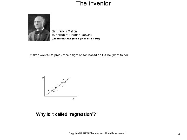
The inventor Sir Francis Galton (A cousin of Charles Darwin) (Source: http: //en. wikipedia. org/wiki/Francis_Galton) Galton wanted to predict the height of son based on the height of father. Why is it called “regression”? Copyright © 2015 Elsevier Inc. All rights reserved. 2

CHAPTER CONTENTS 8. 1 Introduction. . . . . . . 410 8. 2 The Simple Linear Regression Model. . . . 411 8. 3 Inferences on the Least-Squares Estimators. . . . 425 8. 4 Predicting a Particular Value of Y. . . . . 433 8. 5 Correlation Analysis. . . . . . 436 8. 6 Matrix Notation for Linear Regression. . . . 440 8. 7 Regression Diagnostics. . . . . . 446 8. 8 Chapter Summary. . . . . . 449 8. 9 Computer Examples. . . . . . 450 Project for Chapter 8. . . . . . 456 Copyright © 2015 Elsevier Inc. All rights reserved. 3

Definition of “regression” Regress : To go back; return; move backward. Source: https: //www. yourdictionary. com/regress Predicting the height of son based on the height of father Regression 迴歸 n. 1. The process or an instance of regressing, as to a less perfect or less developed s tate. 2. Psychology Reversion to an earlier or less mature pattern of feeling or behavior. 3. Medicine Subsidence of the symptoms or process of a disease. 4. Statistics A technique for predicting the value of a dependent variable as a functio n of one or more independent variables in the presence of random error. 5. Astronomy Retrograde motion of a celestial body. 6. Geology A relative fall in sea level resulting in deposition of terrestrial strata over marine strata. Source: https: //www. thefreedictionary. com/regression Copyright © 2015 Elsevier Inc. All rights reserved. 4

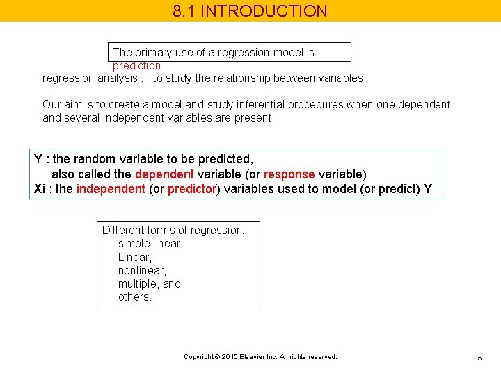
8. 1 INTRODUCTION The primary use of a regression model is prediction regression analysis : to study the relationship between variables Our aim is to create a model and study inferential procedures when one dependent and several independent variables are present. Y : the random variable to be predicted, also called the dependent variable (or response variable) Xi : the independent (or predictor) variables used to model (or predict) Y Different forms of regression: simple linear, Linear, nonlinear, multiple, and others. Copyright © 2015 Elsevier Inc. All rights reserved. 5

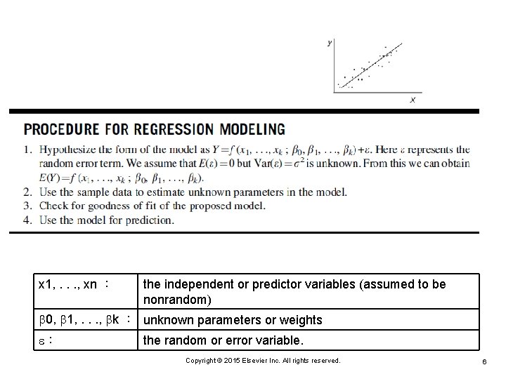
x 1, . . . , xn : the independent or predictor variables (assumed to be nonrandom) 0, 1, . . . , k : unknown parameters or weights : the random or error variable. Copyright © 2015 Elsevier Inc. All rights reserved. 6

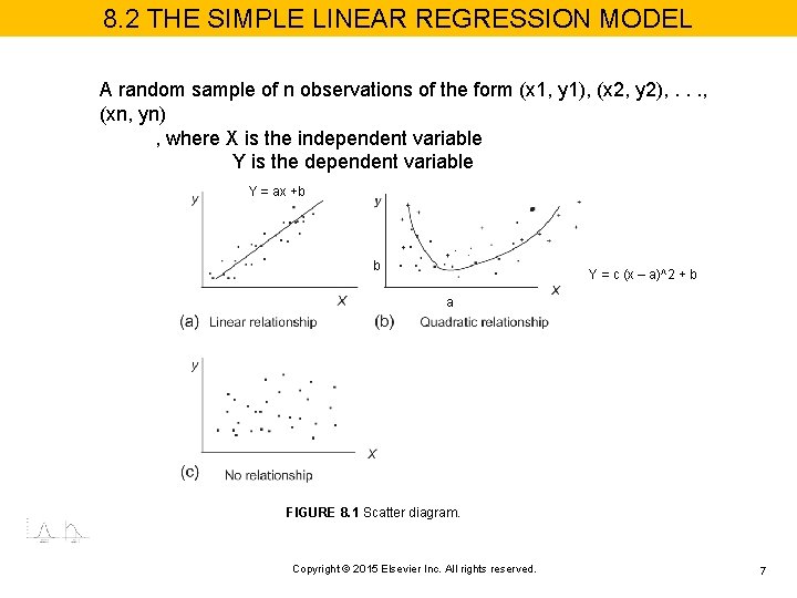
8. 2 THE SIMPLE LINEAR REGRESSION MODEL A random sample of n observations of the form (x 1, y 1), (x 2, y 2), . . . , (xn, yn) , where X is the independent variable Y is the dependent variable Y = ax +b b Y = c (x – a)^2 + b a FIGURE 8. 1 Scatter diagram. Copyright © 2015 Elsevier Inc. All rights reserved. 7

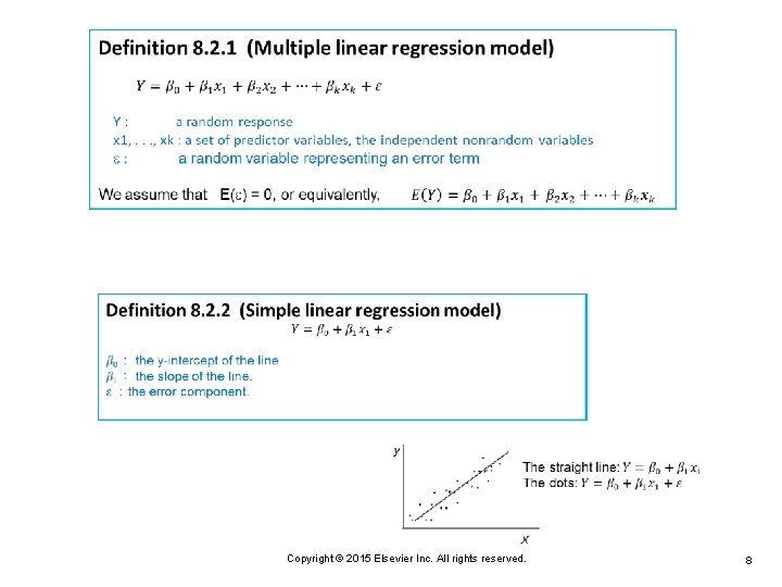
Copyright © 2015 Elsevier Inc. All rights reserved. 8

Copyright © 2015 Elsevier Inc. All rights reserved. 9

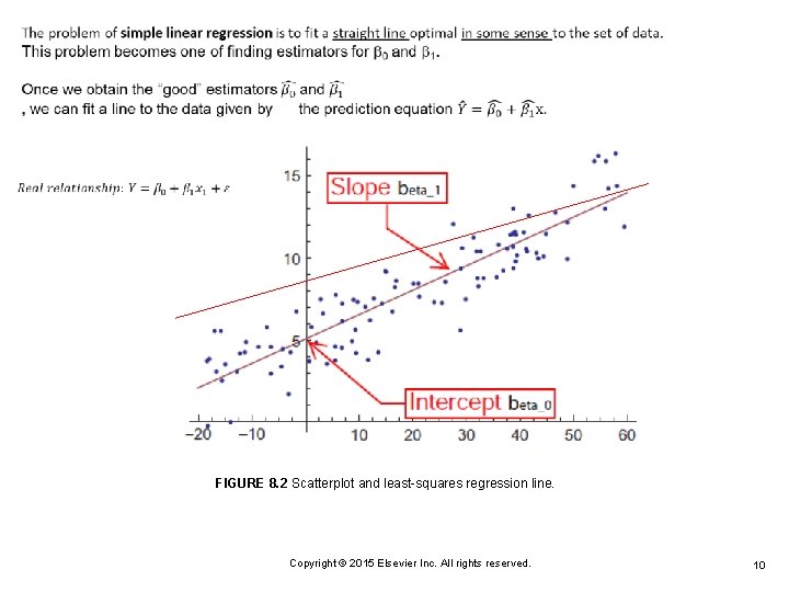
FIGURE 8. 2 Scatterplot and least-squares regression line. Copyright © 2015 Elsevier Inc. All rights reserved. 10

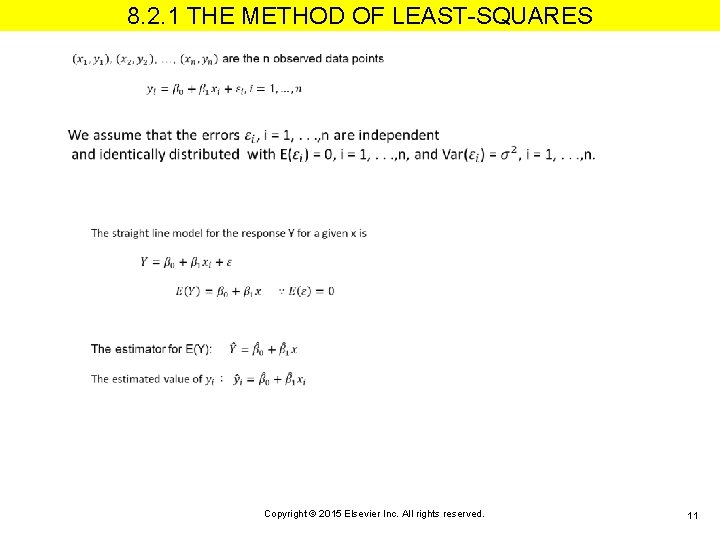
8. 2. 1 THE METHOD OF LEAST-SQUARES Copyright © 2015 Elsevier Inc. All rights reserved. 11

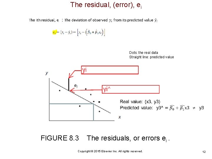
The residual, (error), ei Dots: the real data Straight line: predicted value FIGURE 8. 3 The residuals, or errors ei. Copyright © 2015 Elsevier Inc. All rights reserved. 12

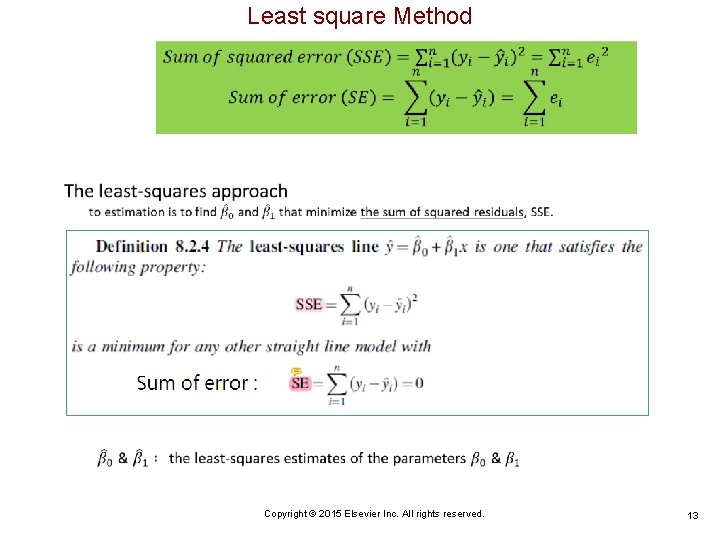
Least square Method Copyright © 2015 Elsevier Inc. All rights reserved. 13

Copyright © 2015 Elsevier Inc. All rights reserved. 14

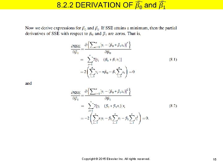
Copyright © 2015 Elsevier Inc. All rights reserved. 15

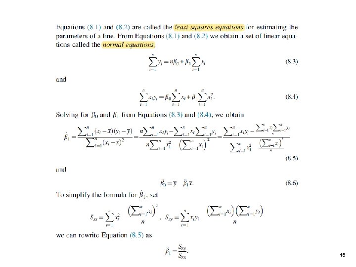
Copyright © 2015 Elsevier Inc. All rights reserved. 16

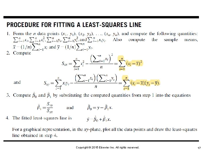
Copyright © 2015 Elsevier Inc. All rights reserved. 17

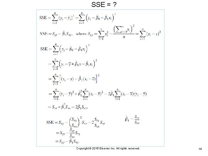
SSE = ? Copyright © 2015 Elsevier Inc. All rights reserved. 18

8. 2. 3 QUALITY OF THE REGRESSION Copyright © 2015 Elsevier Inc. All rights reserved. 19

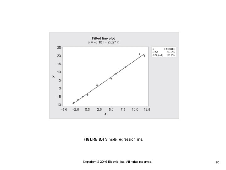
FIGURE 8. 4 Simple regression line. Copyright © 2015 Elsevier Inc. All rights reserved. 20

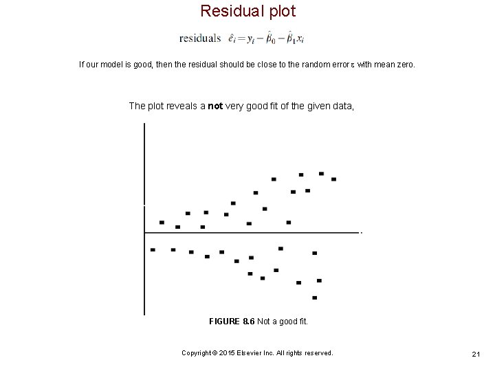
Residual plot If our model is good, then the residual should be close to the random error with mean zero. The plot reveals a not very good fit of the given data, FIGURE 8. 6 Not a good fit. Copyright © 2015 Elsevier Inc. All rights reserved. 21

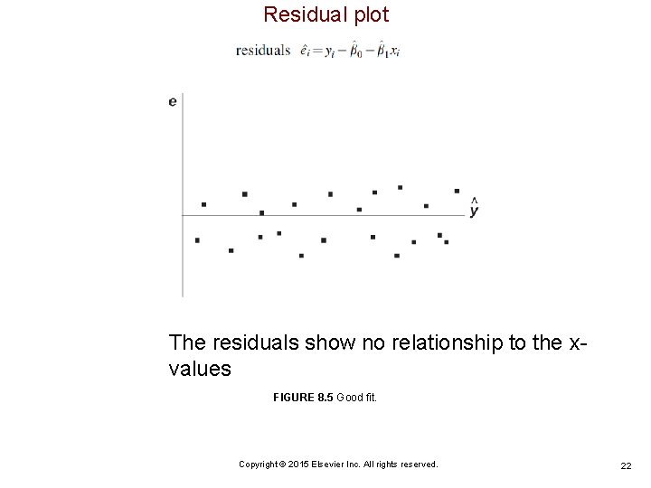
Residual plot The residuals show no relationship to the xvalues FIGURE 8. 5 Good fit. Copyright © 2015 Elsevier Inc. All rights reserved. 22

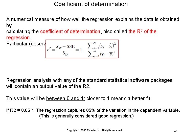
Coefficient of determination A numerical measure of how well the regression explains the data is obtained by calculating the coefficient of determination, also called the R 2 of the regression. Particular (observed) value of realized R 2 is Regression analysis with any of the standard statistical software packages will contain an output value of the R 2. This value will be between 0 and 1; closer to 1 means a better fit. If R 2 = 0. 85: The regression captures 85% of the variation in the dependent variable. (This is generally considered good regression. ) Copyright © 2015 Elsevier Inc. All rights reserved. 23

8. 2. 4 PROPERTIES OF THE LEAST-SQUARES ESTIMATORS FOR THE MODEL Y = 0 + 1 x + Copyright © 2015 Elsevier Inc. All rights reserved. 24

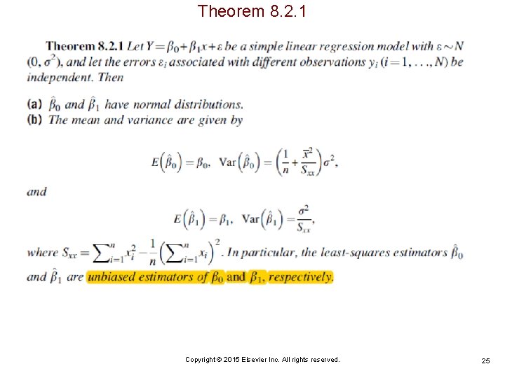
Theorem 8. 2. 1 Copyright © 2015 Elsevier Inc. All rights reserved. 25

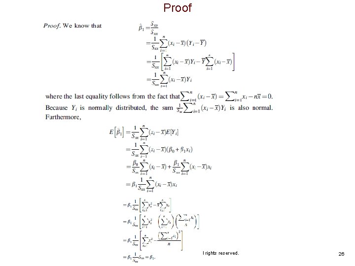
Proof Copyright © 2015 Elsevier Inc. All rights reserved. 26

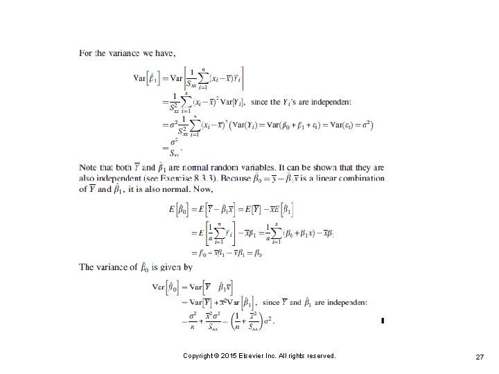
Copyright © 2015 Elsevier Inc. All rights reserved. 27

Copyright © 2015 Elsevier Inc. All rights reserved. 28

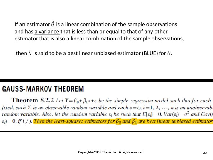
Copyright © 2015 Elsevier Inc. All rights reserved. 29

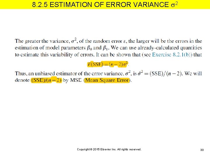
8. 2. 5 ESTIMATION OF ERROR VARIANCE 2 Copyright © 2015 Elsevier Inc. All rights reserved. 30

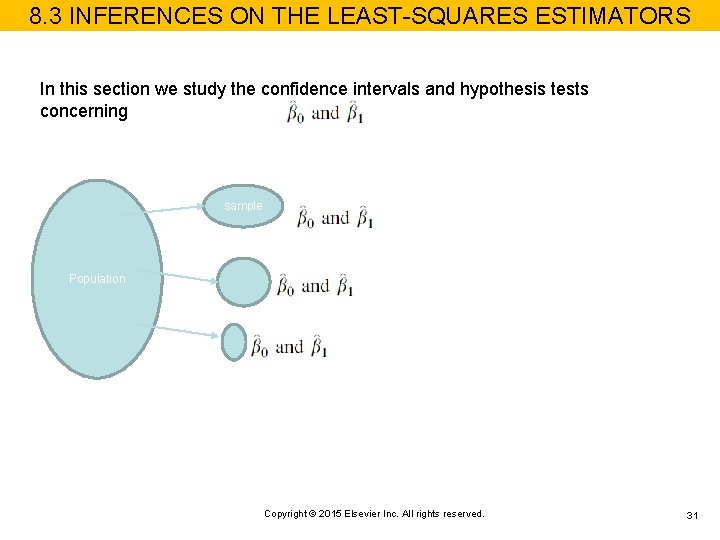
8. 3 INFERENCES ON THE LEAST-SQUARES ESTIMATORS In this section we study the confidence intervals and hypothesis tests concerning sample Population Copyright © 2015 Elsevier Inc. All rights reserved. 31

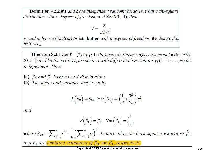
Copyright © 2015 Elsevier Inc. All rights reserved. 32

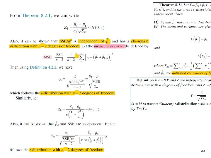
Copyright © 2015 Elsevier Inc. All rights reserved. 33

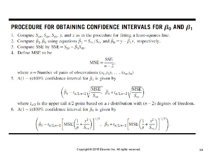
Copyright © 2015 Elsevier Inc. All rights reserved. 34

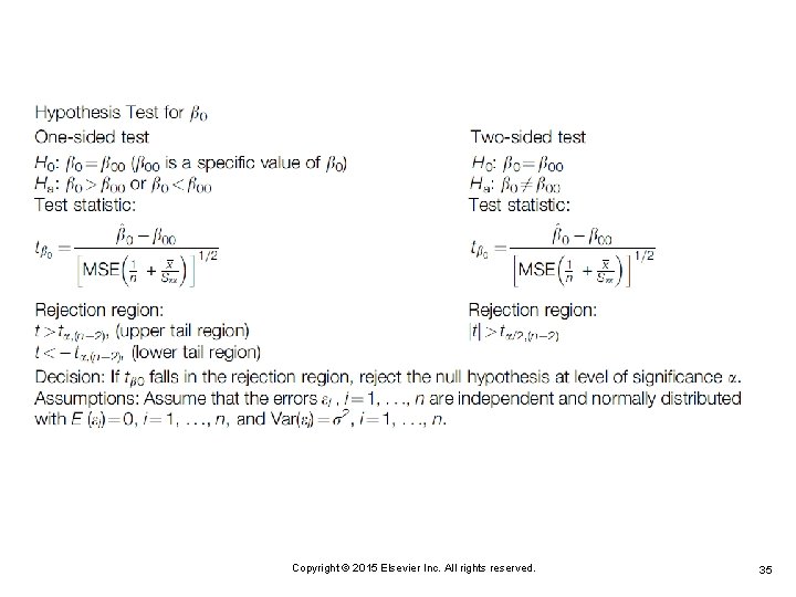
Copyright © 2015 Elsevier Inc. All rights reserved. 35

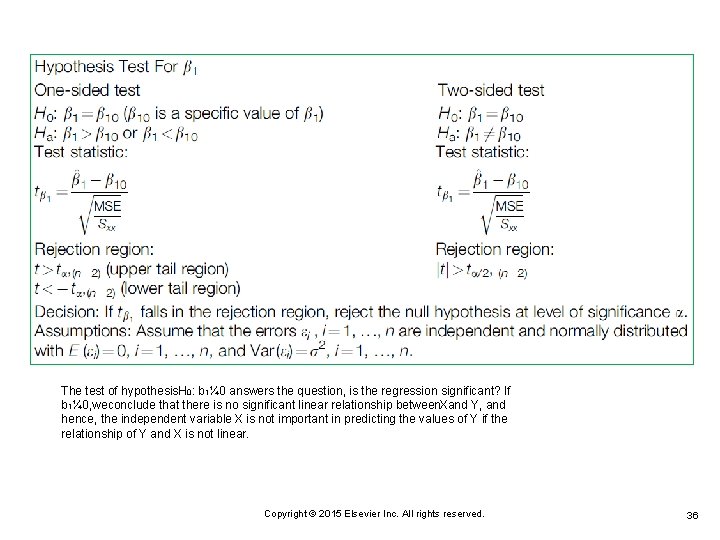
The test of hypothesis. H 0: b 1¼ 0 answers the question, is the regression significant? If b 1¼ 0, weconclude that there is no significant linear relationship between. Xand Y, and hence, the independent variable X is not important in predicting the values of Y if the relationship of Y and X is not linear. Copyright © 2015 Elsevier Inc. All rights reserved. 36

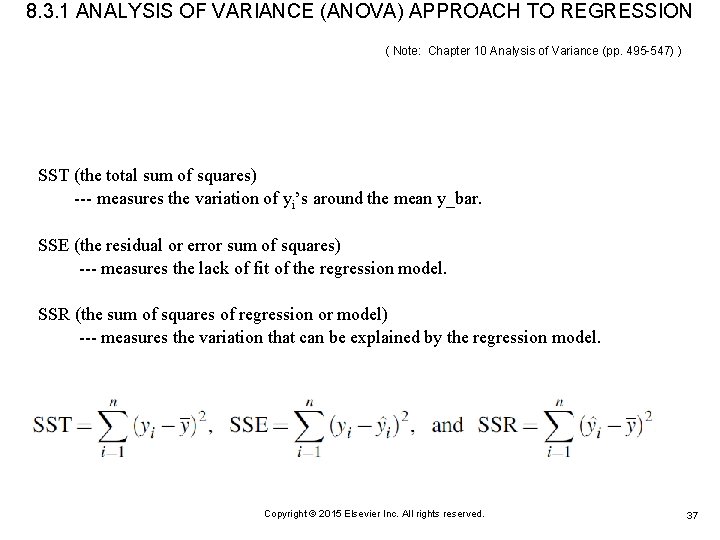
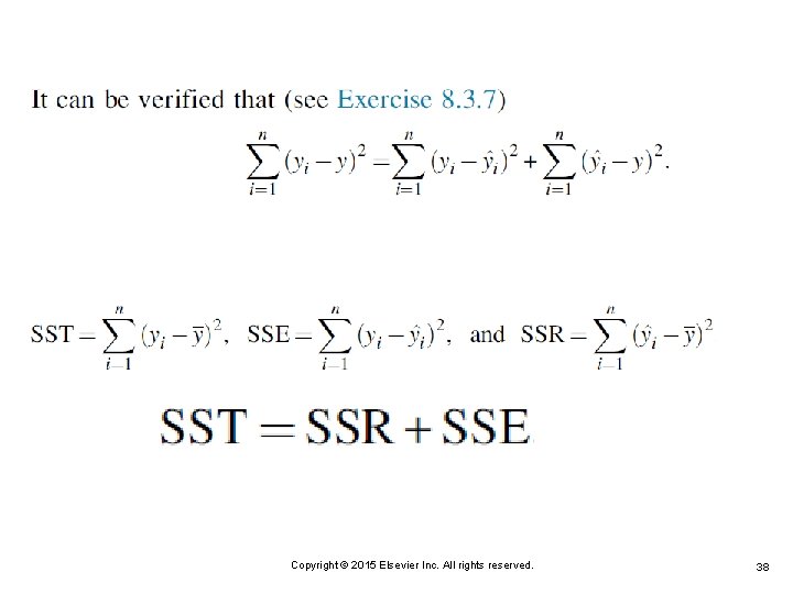
8. 3. 1 ANALYSIS OF VARIANCE (ANOVA) APPROACH TO REGRESSION ( Note: Chapter 10 Analysis of Variance (pp. 495 -547) ) SST (the total sum of squares) --- measures the variation of yi’s around the mean y_bar. SSE (the residual or error sum of squares) --- measures the lack of fit of the regression model. SSR (the sum of squares of regression or model) --- measures the variation that can be explained by the regression model. Copyright © 2015 Elsevier Inc. All rights reserved. 37

Copyright © 2015 Elsevier Inc. All rights reserved. 38

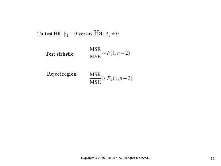
To test H 0: 1 = 0 versus Ha: 1 0 Test statistic: Reject region: Copyright © 2015 Elsevier Inc. All rights reserved. 39

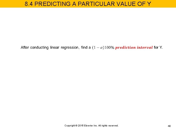
8. 4 PREDICTING A PARTICULAR VALUE OF Y Copyright © 2015 Elsevier Inc. All rights reserved. 40

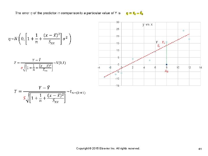
Copyright © 2015 Elsevier Inc. All rights reserved. 41

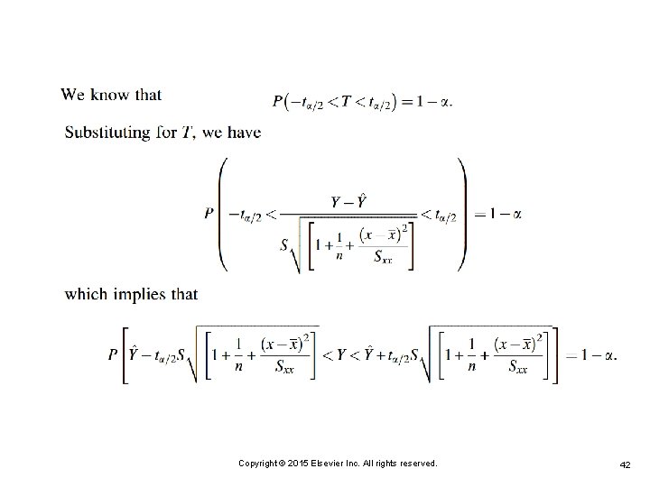
Copyright © 2015 Elsevier Inc. All rights reserved. 42

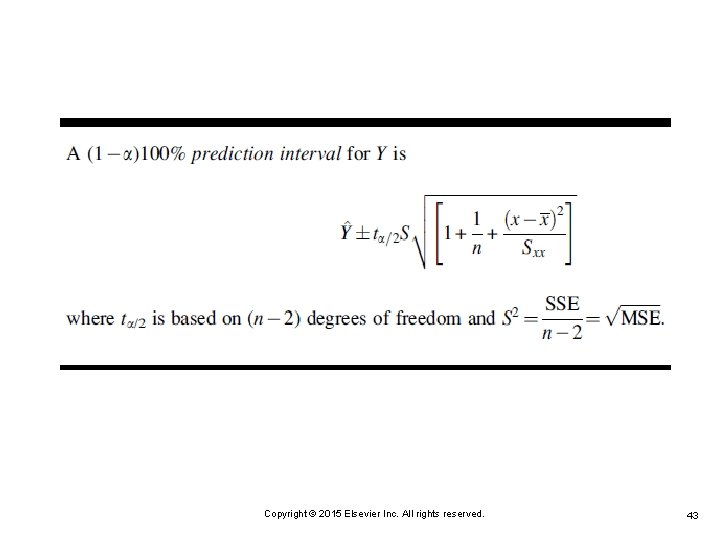
Copyright © 2015 Elsevier Inc. All rights reserved. 43

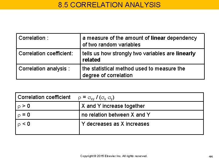
8. 5 CORRELATION ANALYSIS Correlation : a measure of the amount of linear dependency of two random variables Correlation coefficient: tells us how strongly two variables are linearly related Correlation analysis : the statistical method used to measure the degree of correlation Correlation coefficient = xy / ( x y) >0 X and Y increase together =0 no relation between X and Y <0 Y decreases as X increases Copyright © 2015 Elsevier Inc. All rights reserved. 44

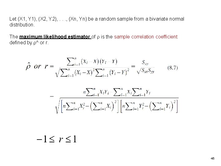
Let (X 1, Y 1), (X 2, Y 2), . . . , (Xn, Yn) be a random sample from a bivariate normal distribution. The maximum likelihood estimator of is the sample correlation coefficient defined by ^ or r. 45

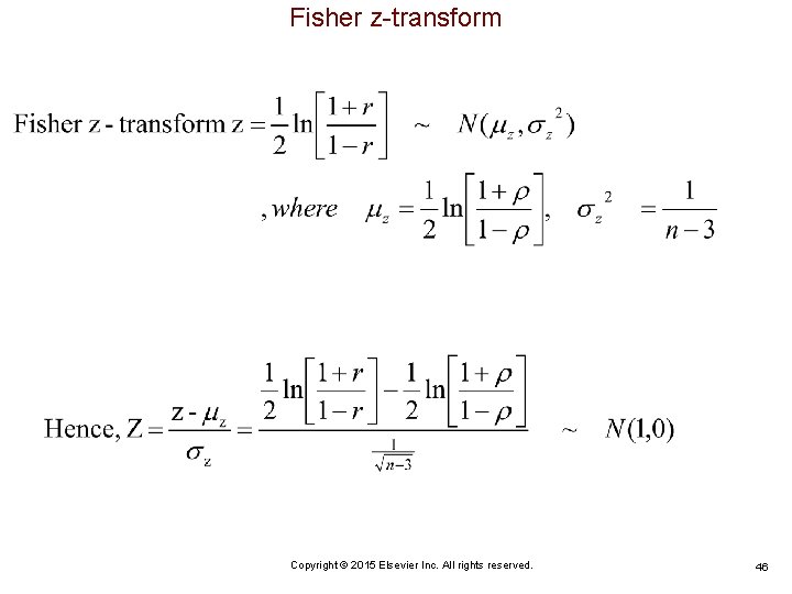
Fisher z-transform Copyright © 2015 Elsevier Inc. All rights reserved. 46

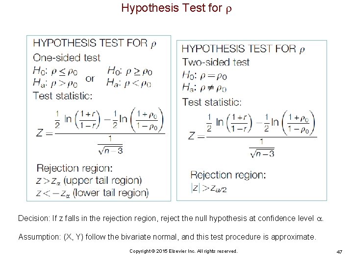
Hypothesis Test for Decision: If z falls in the rejection region, reject the null hypothesis at confidence level . Assumption: (X, Y) follow the bivariate normal, and this test procedure is approximate. Copyright © 2015 Elsevier Inc. All rights reserved. 47

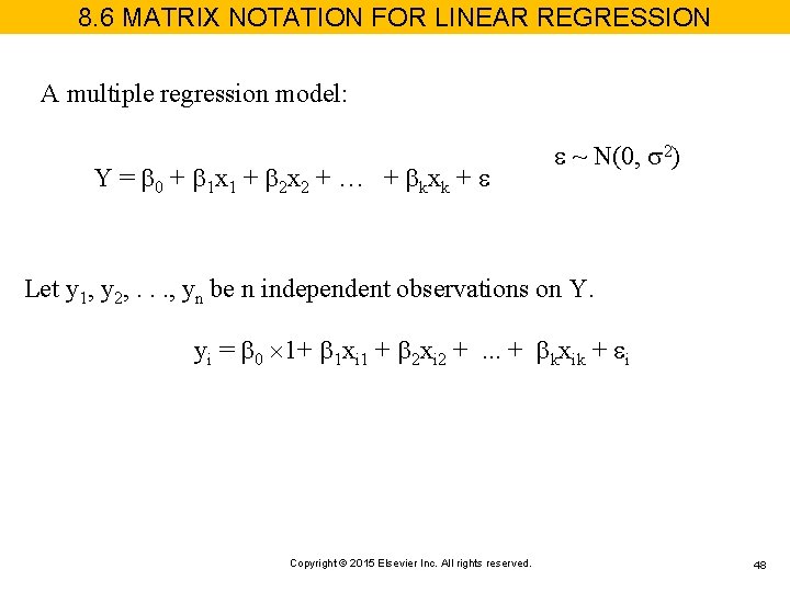
8. 6 MATRIX NOTATION FOR LINEAR REGRESSION A multiple regression model: Y = 0 + 1 x 1 + 2 x 2 + … + kxk + ~ N(0, 2) Let y 1, y 2, . . . , yn be n independent observations on Y. yi = 0 1+ 1 xi 1 + 2 xi 2 +. . . + kxik + i Copyright © 2015 Elsevier Inc. All rights reserved. 48

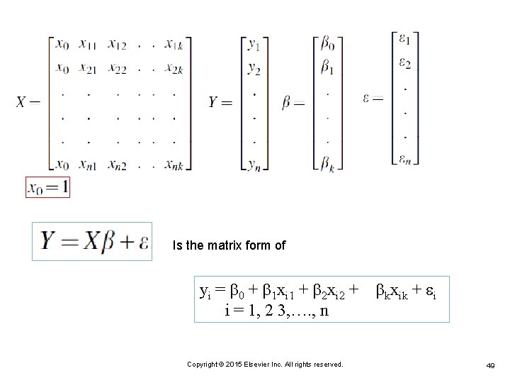
Is the matrix form of yi = 0 + 1 xi 1 + 2 xi 2 + i = 1, 2 3, …. , n Copyright © 2015 Elsevier Inc. All rights reserved. kxik + i 49

Simple linear mode (n = 1) as an example Is equivalent to Copyright © 2015 Elsevier Inc. All rights reserved. 50

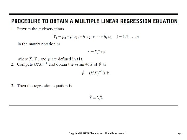
Copyright © 2015 Elsevier Inc. All rights reserved. 51

Copyright © 2015 Elsevier Inc. All rights reserved. 52

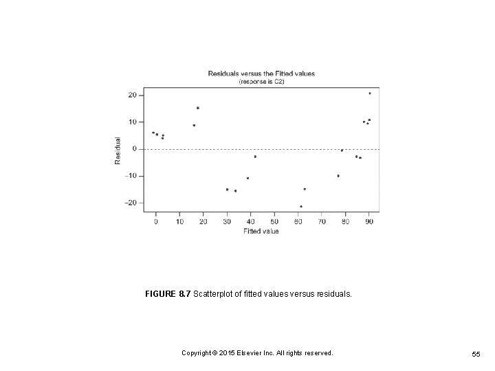
8. 7 REGRESSION DIAGNOSTICS Copyright © 2015 Elsevier Inc. All rights reserved. 53

Copyright © 2015 Elsevier Inc. All rights reserved. 54

FIGURE 8. 7 Scatterplot of fitted values versus residuals. Copyright © 2015 Elsevier Inc. All rights reserved. 55

8. 8 CHAPTER SUMMARY Copyright © 2015 Elsevier Inc. All rights reserved. 56

8. 9 COMPUTER EXAMPLES Copyright © 2015 Elsevier Inc. All rights reserved. 57

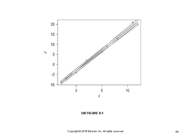
UN FIGURE 8. 1 Copyright © 2015 Elsevier Inc. All rights reserved. 58

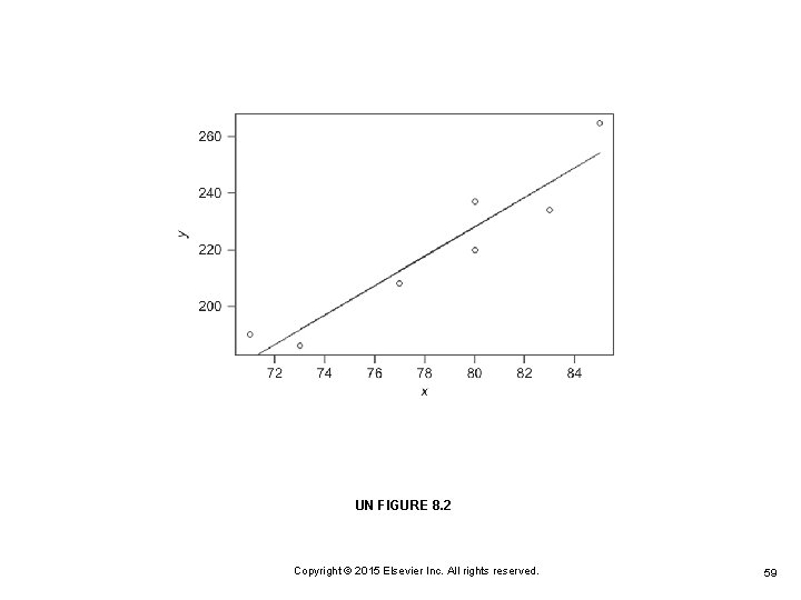
UN FIGURE 8. 2 Copyright © 2015 Elsevier Inc. All rights reserved. 59

Copyright © 2015 Elsevier Inc. All rights reserved. 60