CHAPTER 8 Interest Rate Futures Refinements In this

CHAPTER 8 Interest Rate Futures Refinements In this chapter, we extend the discussion of interest rates futures. This chapter is organized into the following sections: 1. The T Bond Futures Contract 2. Seller’s Options for T Bond Futures 3. Interest Rate Futures Market Efficiency 4. Hedging with T Bond Futures Chapter 8 1

T Bond Futures Contract In this section, the discussion of T bond futures is extended by analyzing the cheapest to deliver bond. Recall that a number of candidate bonds can be delivered against a T bond future contract. Recall further that short traders choose when to deliver and which combination of bonds to deliver. Some bonds are cheaper to obtain than others. In this section, we learn techniques to identify the cheapest to deliver bond, including: 1. Cheapest to deliver bond with no intervening coupons. 2. Cheapest to deliver bond with intervening coupons. 3. Cheapest to deliver and the implied repo rate. Chapter 8 2

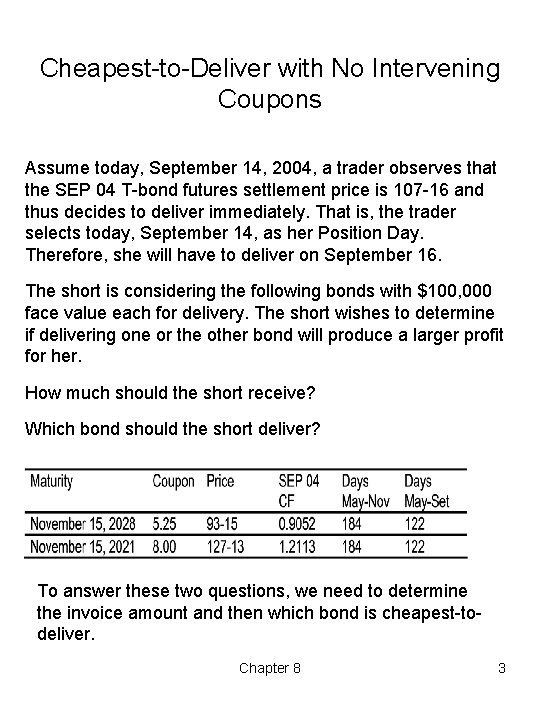
Cheapest to Deliver with No Intervening Coupons Assume today, September 14, 2004, a trader observes that the SEP 04 T bond futures settlement price is 107 16 and thus decides to deliver immediately. That is, the trader selects today, September 14, as her Position Day. Therefore, she will have to deliver on September 16. The short is considering the following bonds with $100, 000 face value each for delivery. The short wishes to determine if delivering one or the other bond will produce a larger profit for her. How much should the short receive? Which bond should the short deliver? To answer these two questions, we need to determine the invoice amount and then which bond is cheapest to deliver. Chapter 8 3

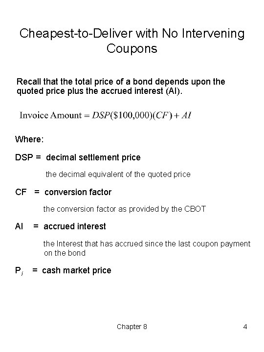
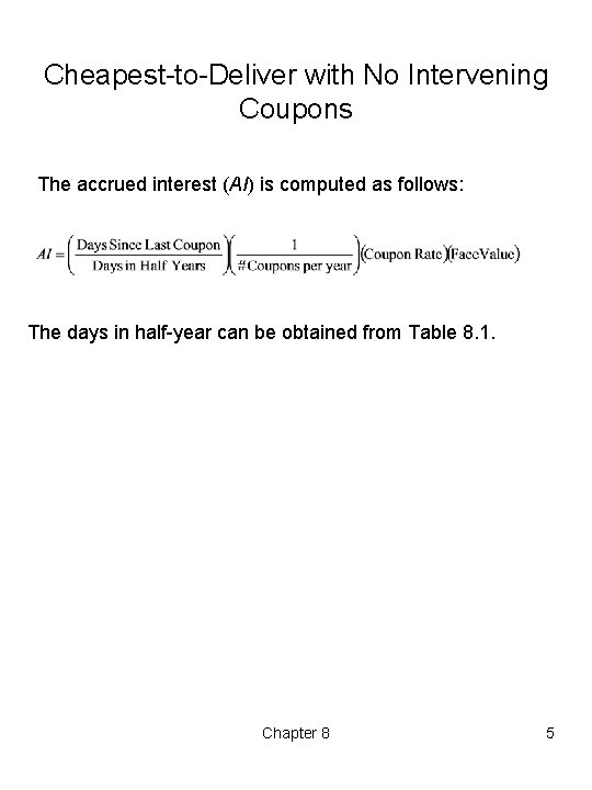
Cheapest to Deliver with No Intervening Coupons Recall that the total price of a bond depends upon the quoted price plus the accrued interest (AI). Where: DSP = decimal settlement price the decimal equivalent of the quoted price CF = conversion factor the conversion factor as provided by the CBOT AI = accrued interest the Interest that has accrued since the last coupon payment on the bond Pi = cash market price Chapter 8 4

Cheapest to Deliver with No Intervening Coupons The accrued interest (AI) is computed as follows: The days in half year can be obtained from Table 8. 1. Chapter 8 5

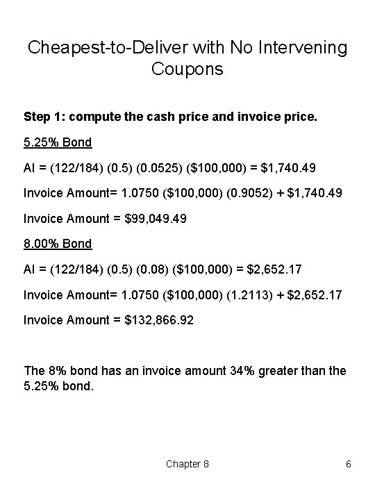
Cheapest to Deliver with No Intervening Coupons Step 1: compute the cash price and invoice price. 5. 25% Bond AI = (122/184) (0. 5) (0. 0525) ($100, 000) = $1, 740. 49 Invoice Amount= 1. 0750 ($100, 000) (0. 9052) + $1, 740. 49 Invoice Amount = $99, 049. 49 8. 00% Bond AI = (122/184) (0. 5) (0. 08) ($100, 000) = $2, 652. 17 Invoice Amount= 1. 0750 ($100, 000) (1. 2113) + $2, 652. 17 Invoice Amount = $132, 866. 92 The 8% bond has an invoice amount 34% greater than the 5. 25% bond. Chapter 8 6

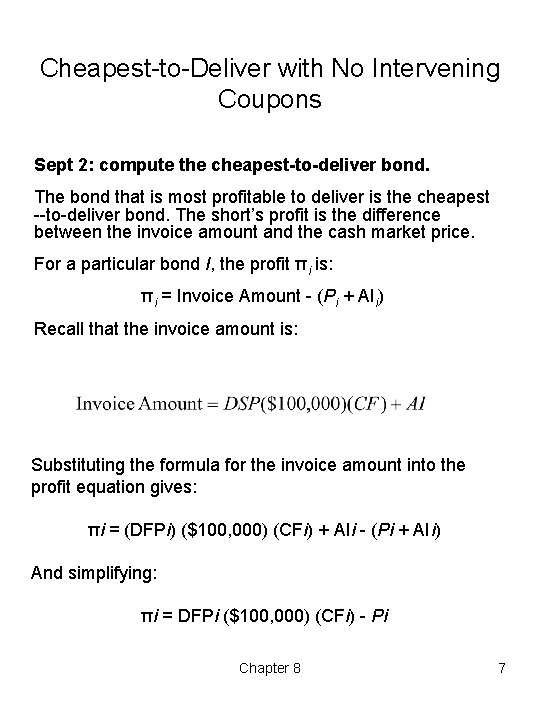
Cheapest to Deliver with No Intervening Coupons Sept 2: compute the cheapest-to-deliver bond. The bond that is most profitable to deliver is the cheapest to deliver bond. The short’s profit is the difference between the invoice amount and the cash market price. For a particular bond I, the profit πi is: πi = Invoice Amount (Pi + AIi) Recall that the invoice amount is: Substituting the formula for the invoice amount into the profit equation gives: πi = (DFPi) ($100, 000) (CFi) + AIi (Pi + AIi) And simplifying: πi = DFPi ($100, 000) (CFi) Pi Chapter 8 7

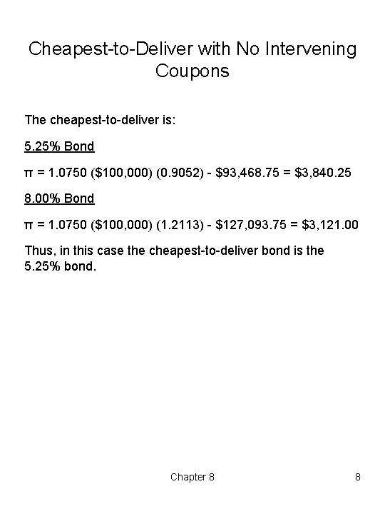
Cheapest to Deliver with No Intervening Coupons The cheapest to deliver is: 5. 25% Bond π = 1. 0750 ($100, 000) (0. 9052) $93, 468. 75 = $3, 840. 25 8. 00% Bond π = 1. 0750 ($100, 000) (1. 2113) $127, 093. 75 = $3, 121. 00 Thus, in this case the cheapest to deliver bond is the 5. 25% bond. Chapter 8 8

Cheapest to Deliver with No Intervening Coupons General rules based on interest rates: 1. When interest rates are below 6%, there is an incentive to deliver short maturity/high coupon bonds. 2. When interest rates exceed 6%, there is an incentive to deliver long maturity/low coupon bonds. General rules based on duration: 1. A trader should deliver low duration bonds when interest rates are below 6%. 2. A trader should deliver high duration bonds when interest rates are above 6%. Chapter 8 9

Cheapest to Deliver with Intervening Coupons This section examines, cheapest to deliver bonds when a bond pays a coupon between the beginning of the cash and carry holding period and the futures expiration. To find the cheapest to deliver bond before expiration, the cash and carry strategy is used. The bond with the greatest profit at delivery from following the cash and carry strategy will be the cheapest to deliver bond. For this analysis Assume that: 1. A trader buys a bond a today and carries it until delivery. 2. Interest rates and futures prices remain constant. 3. Consider the estimated invoice amount plus the estimate of the cash flows associated with carrying the bond to delivery. Chapter 8 10

Cheapest to Deliver with Intervening Coupons The estimated invoice amount depends on three factors: 1. Today's quoted futures price. 2. The conversion factor for the bond we plan to deliver. 3. The accrued interest on the bond at the expiration date. Acquiring and carrying a bond to delivery involves three cash flows as well: 1. The amount paid today to purchase the bond. 2. The finance cost associated with obtaining money today to buy a bond in the future. 3. The receipt and reinvesting of coupon payment. Figure 8. 1 brings all these factors together. Chapter 8 11

Cheapest to Delivery and Bond Yield Insert Figure 8. 1 here Chapter 8 12

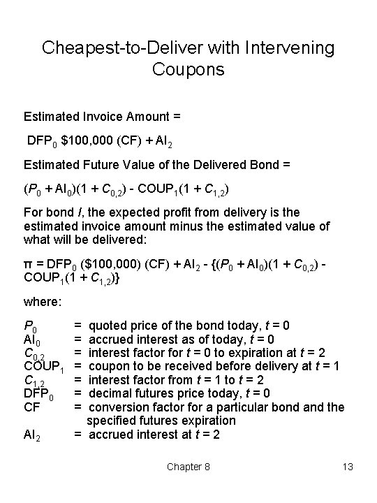
Cheapest to Deliver with Intervening Coupons Estimated Invoice Amount = DFP 0 $100, 000 (CF) + AI 2 Estimated Future Value of the Delivered Bond = (P 0 + AI 0)(1 + C 0, 2) COUP 1(1 + C 1, 2) For bond I, the expected profit from delivery is the estimated invoice amount minus the estimated value of what will be delivered: π = DFP 0 ($100, 000) (CF) + AI 2 {(P 0 + AI 0)(1 + C 0, 2) COUP 1(1 + C 1, 2)} where: P 0 AI 0 C 0, 2 COUP 1 C 1, 2 DFP 0 CF AI 2 = = = = quoted price of the bond today, t = 0 accrued interest as of today, t = 0 interest factor for t = 0 to expiration at t = 2 coupon to be received before delivery at t = 1 interest factor from t = 1 to t = 2 decimal futures price today, t = 0 conversion factor for a particular bond and the specified futures expiration = accrued interest at t = 2 Chapter 8 13

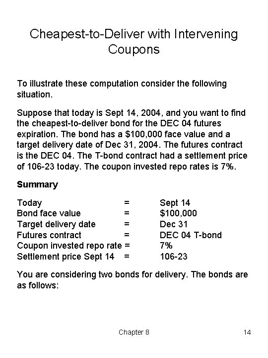
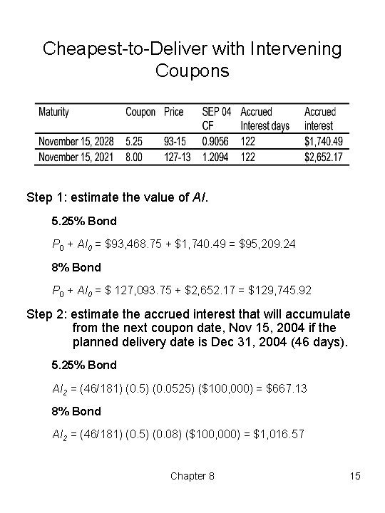
Cheapest to Deliver with Intervening Coupons To illustrate these computation consider the following situation. Suppose that today is Sept 14, 2004, and you want to find the cheapest to deliver bond for the DEC 04 futures expiration. The bond has a $100, 000 face value and a target delivery date of Dec 31, 2004. The futures contract is the DEC 04. The T bond contract had a settlement price of 106 23 today. The coupon invested repo rates is 7%. Summary Today = Bond face value = Target delivery date = Futures contract = Coupon invested repo rate = Settlement price Sept 14 = Sept 14 $100, 000 Dec 31 DEC 04 T bond 7% 106 23 You are considering two bonds for delivery. The bonds are as follows: Chapter 8 14

Cheapest to Deliver with Intervening Coupons Step 1: estimate the value of AI. 5. 25% Bond P 0 + AI 0 = $93, 468. 75 + $1, 740. 49 = $95, 209. 24 8% Bond P 0 + AI 0 = $ 127, 093. 75 + $2, 652. 17 = $129, 745. 92 Step 2: estimate the accrued interest that will accumulate from the next coupon date, Nov 15, 2004 if the planned delivery date is Dec 31, 2004 (46 days). 5. 25% Bond AI 2 = (46/181) (0. 5) (0. 0525) ($100, 000) = $667. 13 8% Bond AI 2 = (46/181) (0. 5) (0. 08) ($100, 000) = $1, 016. 57 Chapter 8 15

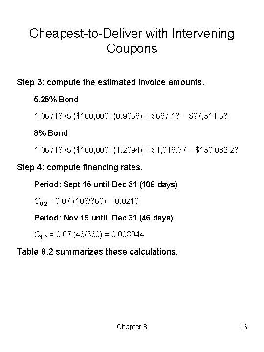
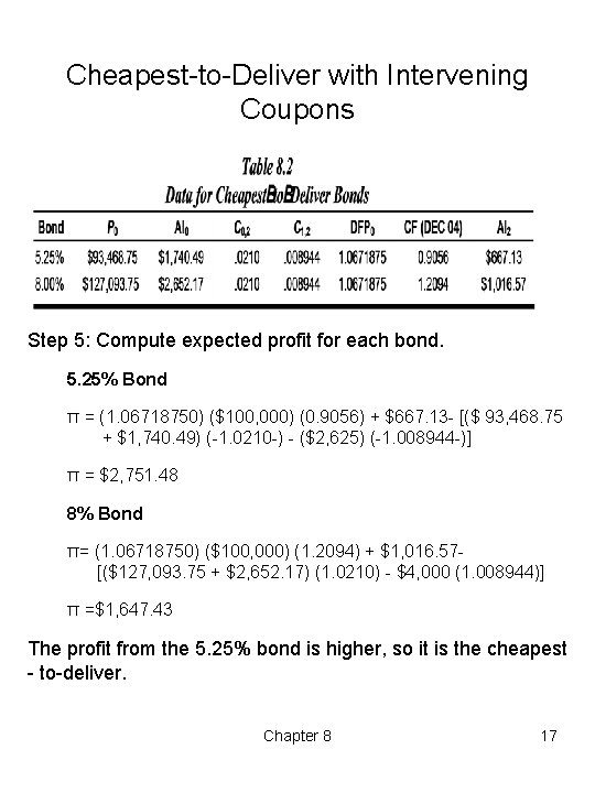
Cheapest to Deliver with Intervening Coupons Step 3: compute the estimated invoice amounts. 5. 25% Bond 1. 0671875 ($100, 000) (0. 9056) + $667. 13 = $97, 311. 63 8% Bond 1. 0671875 ($100, 000) (1. 2094) + $1, 016. 57 = $130, 082. 23 Step 4: compute financing rates. Period: Sept 15 until Dec 31 (108 days) C 0, 2 = 0. 07 (108/360) = 0. 0210 Period: Nov 15 until Dec 31 (46 days) C 1, 2 = 0. 07 (46/360) = 0. 008944 Table 8. 2 summarizes these calculations. Chapter 8 16

Cheapest to Deliver with Intervening Coupons Step 5: Compute expected profit for each bond. 5. 25% Bond π = (1. 06718750) ($100, 000) (0. 9056) + $667. 13 [($ 93, 468. 75 + $1, 740. 49) ( 1. 0210 ) ($2, 625) ( 1. 008944 )] π = $2, 751. 48 8% Bond π= (1. 06718750) ($100, 000) (1. 2094) + $1, 016. 57 [($127, 093. 75 + $2, 652. 17) (1. 0210) $4, 000 (1. 008944)] π =$1, 647. 43 The profit from the 5. 25% bond is higher, so it is the cheapest to deliver. Chapter 8 17

Cheapest to Deliver Bond and The Implied Repo Rate We can analyze the same situation using the implied repo rate. The implied repo rate for a given period equals the net cash flow at delivery divided by the net cash flow when the carry starts. Repo Rate General Rules 1. A cash and carry arbitrage nets a zero profit if the actual borrowing cost equals the implied repo rate. 2. If the effective borrowing rate is less than the implied repo rate, one can earn an arbitrage profit by using cash and carry arbitrage (i. e. , buy a cash bond and sell a futures). 3. If the effective borrowing rate exceeds the implied repo rate and if one can sell bonds short, then one can earn an arbitrage profit by using a reverse cash and carry arbitrage ( i. e. , sell a bond short, buy the futures, and cover the short position at the expiration of the futures). Chapter 8 18

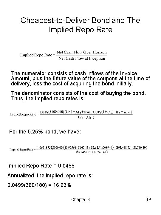
Cheapest to Deliver Bond and The Implied Repo Rate The numerator consists of cash inflows of the Invoice Amount, plus the future value of the coupons at the time of delivery, less the cost of acquiring the bond initially. The denominator consists of the cost of buying the bond. Thus, the Implied repo rates is: For the 5. 25% bond, we have: Implied Repo Rate = 0. 0499 Annualized, the implied repo rate is: 0. 0499(360/180) = 16. 63% Chapter 8 19

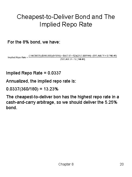
Cheapest to Deliver Bond and The Implied Repo Rate For the 8% bond, we have: Implied Repo Rate = 0. 0337 Annualized, the implied repo rate is: 0. 0337(360/180) = 13. 23% The cheapest to deliver bon has the highest repo rate in a cash and carry arbitrage, so we should deliver the 5. 25% bond. Chapter 8 20

Cheapest to Deliver Bond and Implied Repo Rate Table 8. 3 shows how financing a cash and carry arbitrage at the implied repo rate yields a zero profit. Chapter 8 21

T Bond Risk Arbitrage in the T bond futures market is really risk arbitrage. Risks stem from three sources: 1. Intervening coupon payments that must face reinvestment. 2. The use of conversion factors. 3. The seller options. Chapter 8 22

T Bond Risk Arbitrage A closer examination of Table 8. 3 shows some potentially risky elements of the cash and carry arbitrage. Notice that: 1. The debt was financed at a constant rate throughout the 108 day carry period. 2. The trader was able to invest the coupon at the reinvestment rate of 7%. 3. The futures price did not change over the horizon. Chapter 8 23

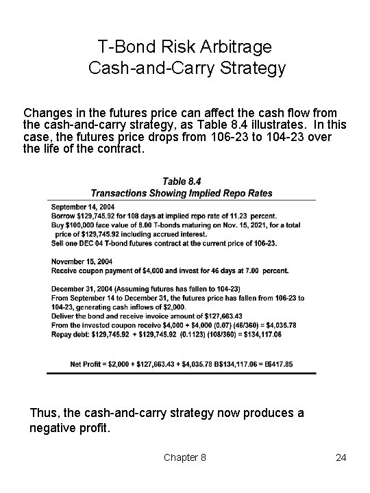
T Bond Risk Arbitrage Cash and Carry Strategy Changes in the futures price can affect the cash flow from the cash and carry strategy, as Table 8. 4 illustrates. In this case, the futures price drops from 106 23 to 104 23 over the life of the contract. Thus, the cash and carry strategy now produces a negative profit. Chapter 8 24

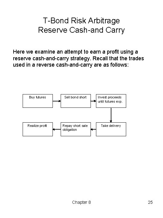
T Bond Risk Arbitrage Reserve Cash and Carry Here we examine an attempt to earn a profit using a reserve cash and carry strategy. Recall that the trades used in a reverse cash and carry are as follows: Buy futures Sell bond short Invest proceeds until futures exp. Realize profit Repay short sale obligation Take delivery Chapter 8 25

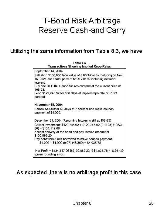
T Bond Risk Arbitrage Reserve Cash and Carry Utilizing the same information from Table 8. 3, we have: As expected , there is no arbitrage profit in this case. Chapter 8 26

T Bond Futures Seller’s Options The structure of T bond futures contract gives sellers timing and quality options. 1. Timing option The seller’s right to choose the time of delivery. 2. Quality option The seller’s right to select which bond to deliver. These two main seller's options become entangled in the actual T bond futures contract. The timing and quality options are commonly present in what the futures markets refers to as: 1. The wildcard option. 2. The end of the month option. Chapter 8 27

Wildcard Option The settlement price is determined at 2: 00 PM. However, the short seller has until 8: 00 PM to notify the exchange of his/her intent to deliver. Thus, the seller can observe what happens between 2: 00 PM and 8: 00 PM before making his/her decision. If interest rates jump between 2: 00 PM and 8: 00 PM, the short trader notifies the exchange his/her intent to deliver at the 2: 00 PM price. If interest rates stay the same or go down, the short seller waits for the next day to notify the exchange of an intent to deliver. Chapter 8 28

The End of the Month Option Recall that the last trading day for T bond futures is the 8 th of the month. The settlement price established on the final trading day is the settlement price used in all invoice calculations for all deliveries in the month. Thus, the seller can still make two choices: 1. The seller can choose the delivery date. 2. The seller can choose the bond to deliver. Assuming that interest rates are stable, then the seller may apply the following general rules: 1. If the coupon yield on the bond exceeds the financing rate to hold the bond, the seller should deliver on the last day. 2. If the financing rate exceeds the coupon yield, the seller should deliver immediately. Chapter 8 29

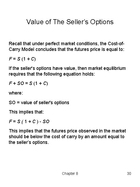
Value of The Seller’s Options Recall that under perfect market conditions, the Cost of Carry Model concludes that the futures price is equal to: F = S (1 + C) If the seller's options have value, then market equilibrium requires that the following equation holds: F + SO = S (1 + C) where: SO = value of seller's options This implies that: F = S ( 1 + C ) SO This implies that the futures price observed in the market should be below the cost of carry by an amount equal to the seller’s options. Chapter 8 30

Interest Rate Futures Market Efficiency There are three commonly distinguished forms of the market efficiency hypothesis: – The weak form. – The semi strong form. – The strong form. While many studies neglect the full magnitude of transaction charges, more recent studies find potential for arbitrage even after transaction costs. Pure Arbitrage For a pure arbitrage, the yield discrepancy must be large enough to cover all transaction costs faced by a market outsider. Quasi Arbitrage Occurs when a trader with an initial portfolio can successfully engage in an arbitrage. For quasi arbitrage, the trader faces less than full transaction costs. Chapter 8 31

Pure Arbitrage Table 8. 9 is from a famous study on the efficiency of the T bill futures market conducted by Elton, Gruber and Rentzler. They found large arbitrage profits exist, many with single contract profits in excess of $800. Chapter 8 32

Pure Arbitrage in T Bond Futures Kolb, Gay and Jordan conducted a study on T bond futures. They investigated the possibility of a pure arbitrage for all T bond contracts from December 1977 through June 1981. Figure 8. 4 shows the profitability of deliverable bond for 15 contracts maturities. Insert Figure 8. 4 here Chapter 8 33

Alternative Risk Management Strategy In this section, alternative risk management strategies using short term interest rate futures are explored, including: 1. Changing the Maturity of an Investment Shortening the maturity of a T bill investment Lengthening the maturity 2. Fixed and Floating Loan Rates 3. Strip and Stack Hedges 4. Tailing Hedge Chapter 8 34

Changing The Maturity of an Investment Shortening the Maturity Many investors find themselves holding a portfolio with undesirable maturity characteristics. Spot market transaction costs are relatively high, and many investors prefer to alter the maturities of investment by trading futures. Consider a firm that has invested in a T bill with a $1, 000 face value. Today, March 20, the T bill has a maturity of 180 days. The firm’s manager learns that the company will need cash in 90 days. Assume that the short term yield is flat with all rates at 10% and a 360 day year. Chapter 8 35

Changing The Maturity of an Investment Shortening the Maturity Table 8. 10 illustrate the process of shortening the maturity. The price of a bill is given by: P = FV [DY(FV)(DTM)]/360 P= $1, 000 [(. 10)($10, 000(180)]/360 P= $1, 000 $50, 000 = $9, 500, 000 By making the above trades, the firm has effectively shortened the maturity from 6 months to three months. Chapter 8 36

Changing The Maturity of an Investment Lengthening the Maturity On August 21, an investor holds a T bill with a $100 million face value. The T bill matures in 30 days (September 20). The investor plans to reinvest for another 3 months after the T bill matures. The investor fears that interest rates might fall. The investor finds the current SEP T Bill futures yield of 9. 8% attractive and would like to lengthen the maturity of the T bill investment. The transaction necessary to do so are presented in Table 8. 11. These transactions locked in a 9. 8% rate over the four months (Aug Dec). Thereby, lengthening the maturity of the individuals investments. Chapter 8 37

Fixed and Floating Loan Rates This section examines: 1. Converting a Floating Rate to a Fixed Rate Loan – How a borrower holding a floating rate loan can effectively convert this loan into a fixed rate loan. 2. Converting a Fixed Rate to a Floating Rate Loan – How a lender who feels compelled to offer fixed rate loans can use the futures markets to make the investment perform like a floating rate loan. Chapter 8 38

Converting a Floating Rate to a Fixed Rate Loan Converting a floating rate loan to a fixed rate loan, also known as creating a synthetic fixed rate loan, occurs when you start with a floating rate loan and transact to fix the interest rate. Today is Sept 20 th, assume that a construction company has planned a project which will take 6 months to complete. The cost of the project is $100, 000. The firm’s bank offers the following conditions on a loan. Rates First 3 months= Last 3 months= LIBOR + 200 basis point DEC 20 LIBOR + 200 basis point The bank insists that the second 3 month rate be based on the LIBOR prevailing 3 months from today. This is a risky preposition for the construction company. Chapter 8 39

Converting a Floating Rate to a Fixed Rate Loan The construction company wishes to lock in a fixed rate loan for the entire period. The company has accumulated the following information: Sept 20 DEC Eurodollar futures LIBOR Loan 7% 7. 3%. 9. 0% 9. 3% These rates give the following cash flows on the loan: Sept 20 Receive principal + $100, 000 Dec 20 Pay interest 2, 250, 000 Mar 20 Pay interest and principal 102, 325, 000 The cash flows for September and December are certain but the cash flow for March is unknown. Using the above information, construct a synthetic fixed rate loan. Chapter 8 40

Converting a Floating Rate to a Fixed Rate Loan To convert to a variable rate loan to a fixed rate loan, the following transaction are completed. By engaging in the above transactions, the company knows with certainty the interest expense that it will pay over the life of the loan. As such, it has created a fixed rate loan. Chapter 8 41

Converting a Fixed Rate to a Floating Rate Loan From the bank’s perspective, it can grant the fixed rate loan. However, doing so exposes the bank to risks. The bank expects to obtain money to make to the loan by borrowing at LIBOR 7% today and 7. 3% for the next quarter, for an average of 7. 15%. The bank makes a fixed rate loan at 9. 15%. The bank sources of funds are as follows: BANK Sep 20 Dec 20 Mar 20 Borrow principal + $100, 000 Make loan to $100, 000 Pay interest $ 1, 750, 000 Receive principal & interest + $104. 575, 000 Pay principal & interest $101, 825, 000 Chapter 8 42

Converting a Fixed Rate to a Floating Rate Loan To reduce its risks and lock in a profit, the bank trades as follows: Thus, the bank has locked in a profit fo $1, 000 ($4, 575, 000 $3, 575, 000). The bank has also effectively crated a fixed rate loan. Chapter 8 43

Strip and Stack Hedges Using the same example. Now assume that the construction company needs a one year loan instead of 6 month loan. The bank sets the rates to be LIBOR plus 200 basis points. The rate will be adjusted every 3 months to reflect any LIBOR rate changes. On September 15, the construction company observes the following rates: Three month LIBOR DEC Eurodollar MAR Eurodollar JUN Eurodollar 7. 00% 7. 30 7. 60 7. 90 The company estimates that it can finance $100, 000 at the following rates, for an average rate of 9. 45%. I Quarter II Quarte r III Quarter IV Quarter 9. 0% 9. 3 9. 6 9. 9 Chapter 8 44

Stack Hedges A stack hedge occurs when futures contracts are concentrated or stacked in a single future expiration. The construction company enters into a stacked hedge by transacting as shown in Table 8. 14. The hedge worked perfectly by locking in the cost of borrowing regardless of the future course of interest rates. Chapter 8 45

Stack Hedges Notice that in the above example all interest rates change by 50 basis points. Stack hedges may perform poorly if interest rates change in differing amounts. That is, the yield curve shifts. Figure 8. 5 illustrates this situation. Insert Figure 8. 5 here Chapter 8 46

Strip Hedge A strip hedge uses an equal number of contracts for each futures expiration over the hedging horizon. By doing so, the futures market hedge is aligned with the actual risk exposure. The transactions necessary to implement a strip hedge are demonstrated in Table 8. 15. The performance of a strip hedge is superior to the stack hedge because the interest rates adjust every quarter. Chapter 8 47

Advantages of Stacked and Striped Hedge Advantages of Stack Hedges 1. Works better when the cash position has a single horizon. 2. Requires trading a single contract. 3. Advantage of Strip Hedges 4. Can provide a more aligned hedge and better results with a multiple maturity cash position. Chapter 8 48

Tailing The Hedge In a tailing hedge the trader slightly adjusts the hedge to compensate for the interest that can be earned from daily resettlement profits or paid on daily resettlement losses. Thus, the tail of the hedge is the slight reduction in the hedge position to offset the effect of daily resettlement interest. Tail Factor The tail factor is the present value of $1 at the hedging horizon discounted to the present (plus one day) at the investment rate for the resettlement cash flows. Tailed Hedge = Untailed Hedge Tailing Factor. Chapter 8 49

Hedging with T Bond Futures The effectiveness of a hedge depends on the gain or loss on both the spot and futures sides of the transaction. The change in the price of any bond depends on the shifts in the levels of: – Interest rates – Changes in the shape of the yield curve – The maturity of the bond – Bond coupon rate Table 8. 16 and 8. 17 illustrate to effect of maturity and coupon rates on hedging performance. Chapter 8 50

Hedging with T Bond Futures A manager learns on March 1 that he will receive $5 million on June 1 to invest in AAA corporate bonds with a 5% coupon rate and 10 years to maturity. The yield curve is flat and will remain so. The current yield on AAA bonds as well as forward rates are 7. 5%. So the manager expects to acquire the bonds at 7. 5%. However, fearing a drop in rates, he decides to hedge in the futures market to lock in the forward rate of 7. 5%. The manager considers hedging with T bills or T bonds. The AAA bonds have a 5% coupon rate and a 10 year maturity, which do not match the characteristics of either the T bill or T bond futures contracts. The deliverable T bills have a zero coupon and a maturity of only 90 days, and the T bonds have a maturity of at least 15 years and an assortment of semi annual coupons. Assume that the cheapest to deliver T bond will have a 20 year maturity at the target date of June 1, and a 6% coupon. The manager will hedge the AAA position with T bill or T bond futures with yields of 6 and 6. 5%, respectively. The manager plans to invest in 6, 051 bonds each with a price of $826. 30. Chapter 8 51

Hedging with T Bond Futures Table 8. 16 illustrates the transactions and results of hedging with T bill futures. Notice that this loss occurs despite the fact that rates changed by the same amount on both investments. Chapter 8 52

Hedging with T Bond Futures Table 8. 17 illustrates the results of hedging with T bond futures. Again the hedge did not produce the desired results of isolating the portfolio. Chapter 8 53

Hedging with T Bond Futures Simple approaches to hedging interest rate risk often give unsatisfactory results due to mismatches of coupon and maturity characteristics, as demonstrated in the previous examples. This section examines some of the major alternative strategies for hedging interest rate risk: – Face Value Naive (FVN) Model – Market Value Naive (MVN) Model – Conversion Factor (CF) Model – Basis Point (BP) Model – Regression (RGR) Model – Price Sensitivity (PS) Model Chapter 8 54

Face Value Naive (FVN) Model According to FVN Model, the hedger should hedge $1 of face value of the cash instrument with $1 face value of the futures contract. Disadvantages Neglects potential differences in market values between the cash and futures positions. Neglects the coupon and maturity characteristics that affect duration for both the cash market good and the futures contract. Chapter 8 55

Market Value Naïve (MVN) Model The MVN Model recommends hedging $1 of market value in the cash good with $1 of market value in the futures market. Disadvantages Neglects to make adjustments for price sensitivity. Advantages Consider potential differences in market values between cash and futures positions. Chapter 8 56

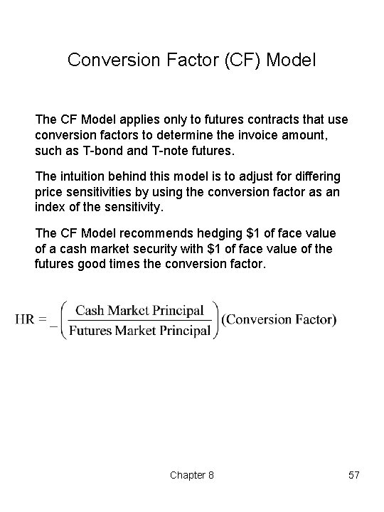
Conversion Factor (CF) Model The CF Model applies only to futures contracts that use conversion factors to determine the invoice amount, such as T bond and T note futures. The intuition behind this model is to adjust for differing price sensitivities by using the conversion factor as an index of the sensitivity. The CF Model recommends hedging $1 of face value of a cash market security with $1 of face value of the futures good times the conversion factor. Chapter 8 57

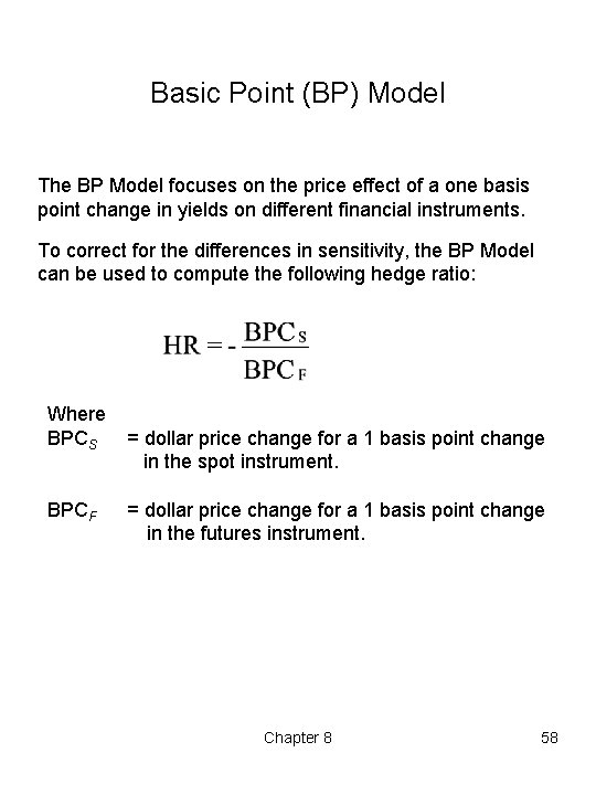
Basic Point (BP) Model The BP Model focuses on the price effect of a one basis point change in yields on different financial instruments. To correct for the differences in sensitivity, the BP Model can be used to compute the following hedge ratio: Where BPCS BPCF = dollar price change for a 1 basis point change in the spot instrument. = dollar price change for a 1 basis point change in the futures instrument. Chapter 8 58

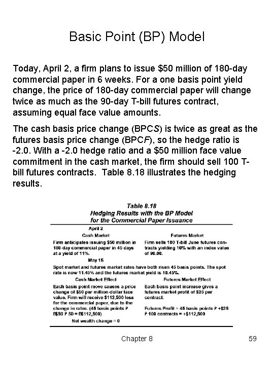
Basic Point (BP) Model Today, April 2, a firm plans to issue $50 million of 180 day commercial paper in 6 weeks. For a one basis point yield change, the price of 180 day commercial paper will change twice as much as the 90 day T bill futures contract, assuming equal face value amounts. The cash basis price change (BPCS) is twice as great as the futures basis price change (BPCF), so the hedge ratio is 2. 0. With a 2. 0 hedge ratio and a $50 million face value commitment in the cash market, the firm should sell 100 T bill futures contracts. Table 8. 18 illustrates the hedging results. Chapter 8 59

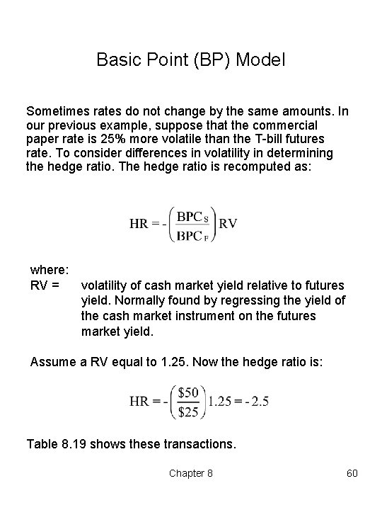
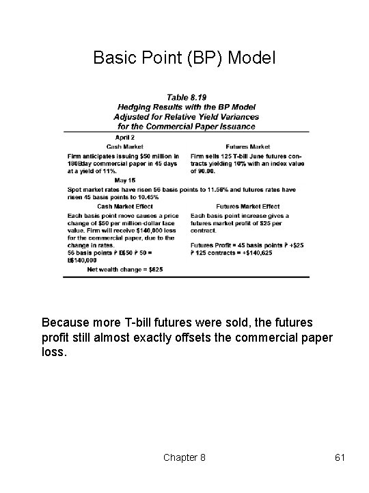
Basic Point (BP) Model Sometimes rates do not change by the same amounts. In our previous example, suppose that the commercial paper rate is 25% more volatile than the T bill futures rate. To consider differences in volatility in determining the hedge ratio. The hedge ratio is recomputed as: where: RV = volatility of cash market yield relative to futures yield. Normally found by regressing the yield of the cash market instrument on the futures market yield. Assume a RV equal to 1. 25. Now the hedge ratio is: Table 8. 19 shows these transactions. Chapter 8 60

Basic Point (BP) Model Because more T bill futures were sold, the futures profit still almost exactly offsets the commercial paper loss. Chapter 8 61

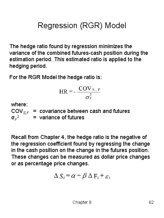
Regression (RGR) Model The hedge ratio found by regression minimizes the variance of the combined futures cash position during the estimation period. This estimated ratio is applied to the hedging period. For the RGR Model the hedge ratio is: where: COVS, F = covariance between cash and futures σF 2 = variance of futures Recall from Chapter 4, the hedge ratio is the negative of the regression coefficient found by regressing the change in the cash position on the change in the futures position. These changes can be measured as dollar price changes or as percentage price changes. Chapter 8 62

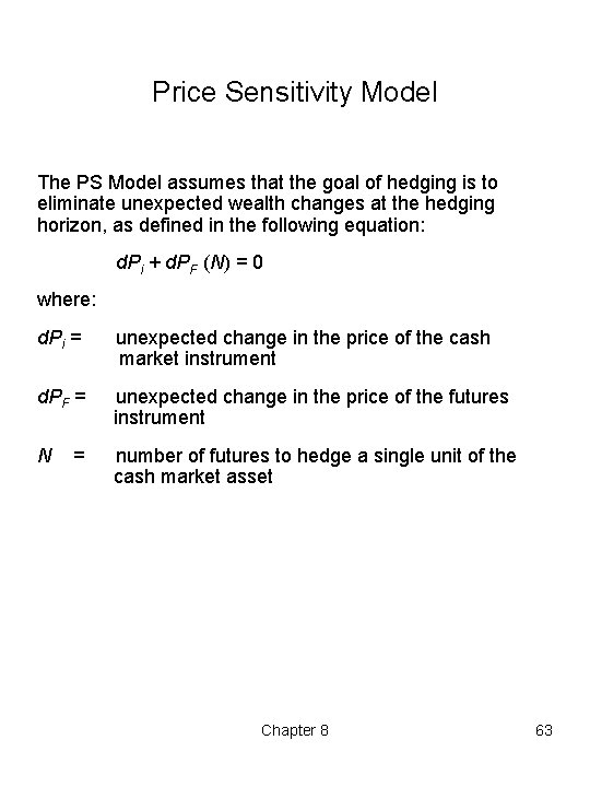
Price Sensitivity Model The PS Model assumes that the goal of hedging is to eliminate unexpected wealth changes at the hedging horizon, as defined in the following equation: d. Pi + d. PF (N) = 0 where: d. Pi = unexpected change in the price of the cash market instrument d. PF = unexpected change in the price of the futures instrument N number of futures to hedge a single unit of the cash market asset = Chapter 8 63

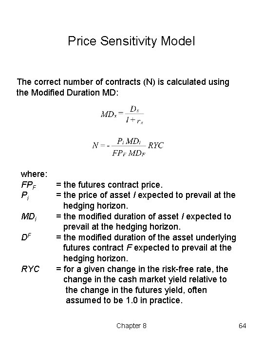
Price Sensitivity Model The correct number of contracts (N) is calculated using the Modified Duration MD: where: FPF Pi MDi DF RYC = the futures contract price. = the price of asset I expected to prevail at the hedging horizon. = the modified duration of the asset underlying futures contract F expected to prevail at the hedging horizon. = for a given change in the risk free rate, the change in the cash market yield relative to the change in the futures yield, often assumed to be 1. 0 in practice. Chapter 8 64

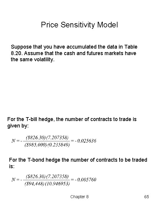
Price Sensitivity Model Suppose that you have accumulated the data in Table 8. 20. Assume that the cash and futures markets have the same volatility. For the T bill hedge, the number of contracts to trade is given by: For the T bond hedge the number of contracts to be traded is: Chapter 8 65

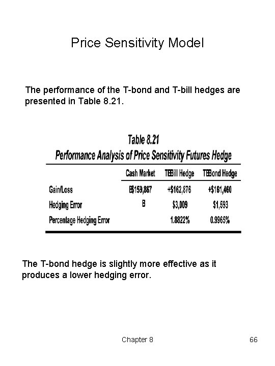
Price Sensitivity Model The performance of the T bond and T bill hedges are presented in Table 8. 21. The T bond hedge is slightly more effective as it produces a lower hedging error. Chapter 8 66

Summary of Alternative Hedging Strategies Chapter 8 67

Immunization In bond investing, maturity mismatches result in exposure to interest rate risk. Consider the case of a bank. when the asset duration is higher than the liability duration, a sudden rise in interest rates will cause the value of the portfolio to decline. When the asset duration is less than the liability duration a sudden rise in interest rates will cause the value of the portfolio to rise. By matching the duration of asset and liabilities, it is possible for the bank to immunize itself from changes in interest rates. We consider two examples of immunization: 1. Planning Period Case 2. Bank Immunization case Chapter 8 68

Immunization with Interest Rate Futures Planning Period Case A portfolio manager has collected the following information: The portfolio manager has a $100 million bond portfolio of bond C with a duration of 9. 2853 years and is considering two alternatives. The manager has a 6 year planning period. The manager wants to shorten the portfolio duration to six years to match the planning period, and is considering two alternatives to do so. Chapter 8 69

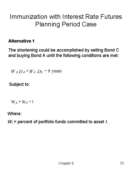
Immunization with Interest Rate Futures Planning Period Case Alternative 1 The shortening could be accomplished by selling Bond C and buying Bond A until the following conditions are met: Subject to: Where: WI = percent of portfolio funds committed to asset I. Chapter 8 70

Immunization with Interest Rate Futures Planning Period Case Alternative 2 The manager could also adjust the portfolio's duration to match the six year planning period by trading interest rate futures and keeping bond C. If bond C and a T bill futures comprise the portfolio, the T bill futures position must satisfy the condition: PP = PC NC + FPT bill NT bill where: Pp Pc FPT bill Nc NT bill = = = value of the portfolio price of bond C t bill futures price number of C bonds number of T bills Expressing the change in the price of a bond as a function of duration and the yield on the asset: d. P = D{d(1 + r)/(1 + r)}P Chapter 8 71

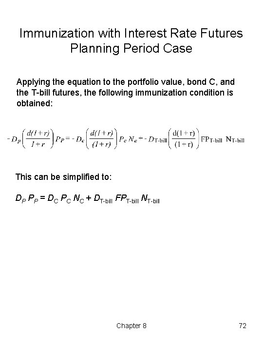
Immunization with Interest Rate Futures Planning Period Case Applying the equation to the portfolio value, bond C, and the T bill futures, the following immunization condition is obtained: This can be simplified to: DP PP = DC PC NC + DT bill FPT bill NT bill Chapter 8 72

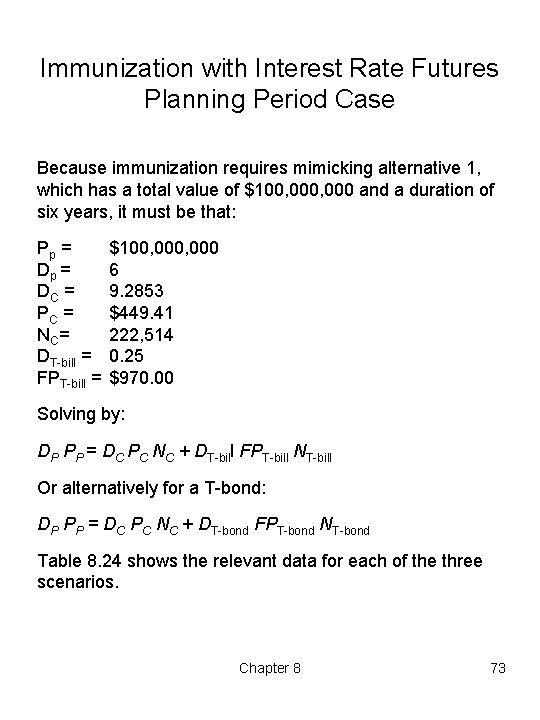
Immunization with Interest Rate Futures Planning Period Case Because immunization requires mimicking alternative 1, which has a total value of $100, 000 and a duration of six years, it must be that: Pp = DC = PC = NC = DT bill = FPT bill = $100, 000 6 9. 2853 $449. 41 222, 514 0. 25 $970. 00 Solving by: DP PP = DC PC NC + DT bill FPT bill NT bill Or alternatively for a T bond: DP PP = DC PC NC + DT bond FPT bond NT bond Table 8. 24 shows the relevant data for each of the three scenarios. Chapter 8 73

Immunization with Interest Rate Futures Planning Period Case Chapter 8 74

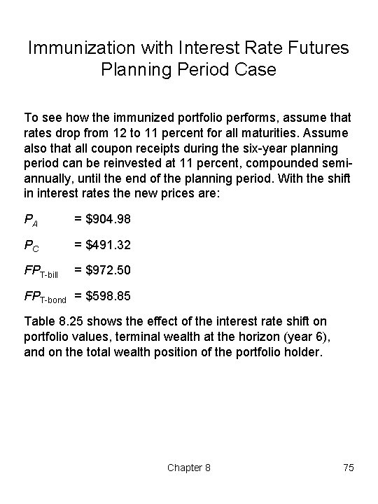
Immunization with Interest Rate Futures Planning Period Case To see how the immunized portfolio performs, assume that rates drop from 12 to 11 percent for all maturities. Assume also that all coupon receipts during the six year planning period can be reinvested at 11 percent, compounded semi annually, until the end of the planning period. With the shift in interest rates the new prices are: PA = $904. 98 PC = $491. 32 FPT bill = $972. 50 FPT bond = $598. 85 Table 8. 25 shows the effect of the interest rate shift on portfolio values, terminal wealth at the horizon (year 6), and on the total wealth position of the portfolio holder. Chapter 8 75

Immunization with Interest Rate Futures Planning Period Case Notice that each portfolio responds similarly. Chapter 8 76

Transaction Costs for Planning Period Case While each of the portfolios are equally effective in immunizing, the cost of obtaining the immunization varies as demonstrated in Table 8. 28. Notice that the cost of becoming immunized varies from $949, 315 to $13, 240 depending upon the strategy selected. Chapter 8 77

Immunization with Interest Rate Futures Bank Immunization Case Assume that a bank holds a $100, 000 liability portfolio in Bond B, the composition of which is fixed. The bank wishes to hold an asset portfolio of Bonds A and C that will protect the wealth position of the bank from any change as a result of a change in yields. Five different portfolio combinations illustrate different means to achieve the desired result: Portfolio 1: Hold Bond A and Bond C (the traditional approach) Portfolio 2: Hold Bond C; Sell T bill futures Portfolio 3: Hold Bond A; Buy T bond futures Portfolio 4: Hold Bond A; Buy T bill futures Portfolio 5: Hold Bond C; Sell T bond futures The portfolios are presented in Table 8. 26. For each portfolio, the full $100, 000 is put into a bond portfolio and is balanced out by cash. Chapter 8 78

Immunization with Interest Rate Futures Bank Immunization Case Chapter 8 79

Immunization with Interest Rate Futures Bank Immunization Case Now consider a drop in rates from 12% to 11% for all maturities. The effect on the portfolio is presented in Table 8. 27. Notice that all 5 methods perform similarly. Chapter 8 80