Chapter 8 Inferences from Two Samples Slide 1

Chapter 8 Inferences from Two Samples Slide 1 8 -1 Overview 8 -2 Inferences about Two Proportions 8 -3 Inferences about Two Means: Independent Samples 8 -4 Inferences about Matched Pairs 8 -5 Comparing Variation in Two Samples Chapter 8, Triola, Elementary Statistics, MATH 1342

Slide 2 Section 8 -1 & 8 -2 Overview and Inferences about Two Proportions Created by Erin Hodgess, Houston, Texas

Overview (p. 438) Slide 3 There are many important and meaningful situations in which it becomes necessary to compare two sets of sample data. Chapter 8, Triola, Elementary Statistics, MATH 1342

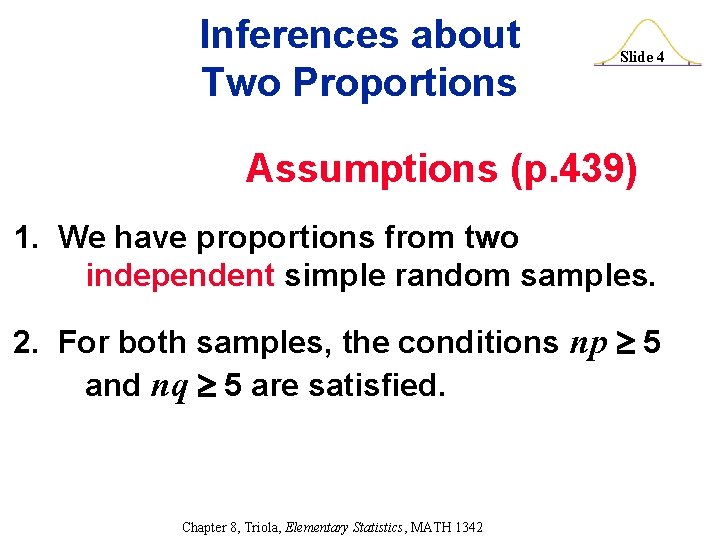
Inferences about Two Proportions Slide 4 Assumptions (p. 439) 1. We have proportions from two independent simple random samples. 2. For both samples, the conditions np 5 and nq 5 are satisfied. Chapter 8, Triola, Elementary Statistics, MATH 1342

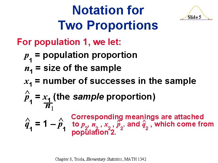
Notation for Two Proportions Slide 5 For population 1, we let: p 1 = population proportion n 1 = size of the sample x 1 = number of successes in the sample ^ p = x 1 (the sample proportion) 1 n 1 q^1 = 1 – Corresponding meanings are attached p^1 to p 2, n 2 , x 2 , ^p 2. and ^q 2 , which come from population 2. Chapter 8, Triola, Elementary Statistics, MATH 1342

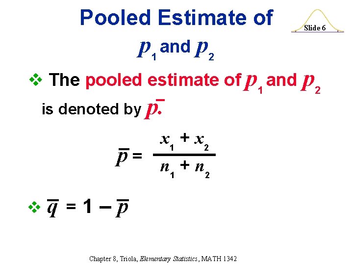
Pooled Estimate of p 1 and p 2 v The pooled estimate of p 1 and is denoted by p. x 1 + x 2 p= n +n 1 2 v q =1–p Chapter 8, Triola, Elementary Statistics, MATH 1342 Slide 6 p 2

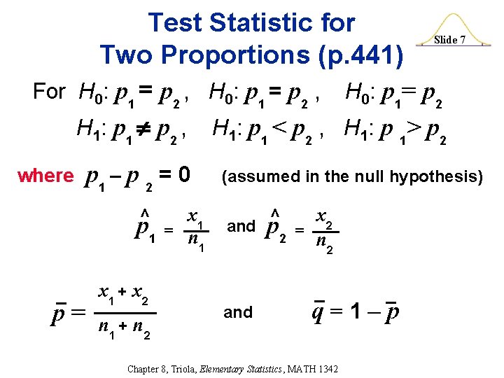
Test Statistic for Two Proportions (p. 441) For H 0: p 1 = p 2 , H 1: p 1 p 2 , where p 1 – p 2 = 0 p^ 1 p= x 1 + x 2 n 1 + n 2 x 1 = n 1 Slide 7 H 0: p 1= p 2 H 1: p 1 < p 2 , H 1: p 1> p 2 (assumed in the null hypothesis) and p^ 2 x 2 = n 2 q=1–p Chapter 8, Triola, Elementary Statistics, MATH 1342

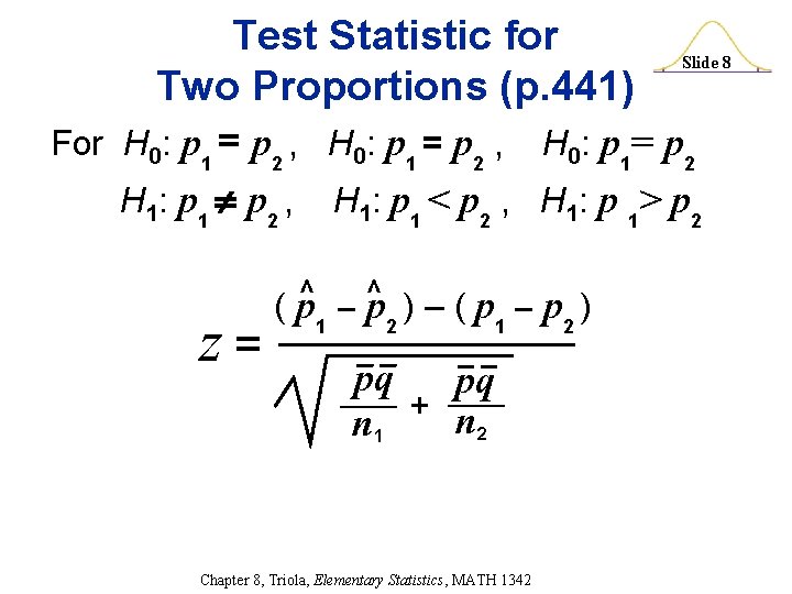
Test Statistic for Two Proportions (p. 441) For H 0: p 1 = p 2 , H 1: p 1 p 2 , z= Slide 8 H 0: p 1= p 2 H 1: p 1 < p 2 , H 1: p 1> p 2 ^ )–(p –p ) ( p^1 – p 2 1 2 pq pq n 1 + n 2 Chapter 8, Triola, Elementary Statistics, MATH 1342

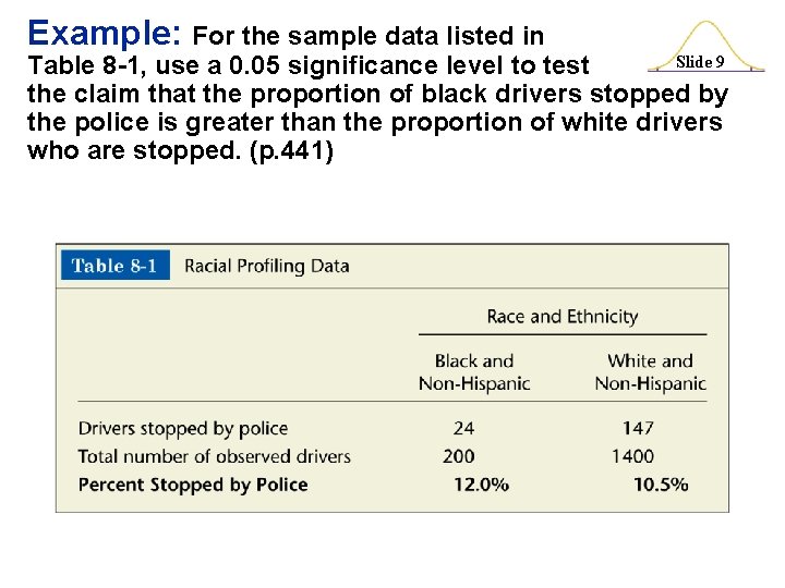
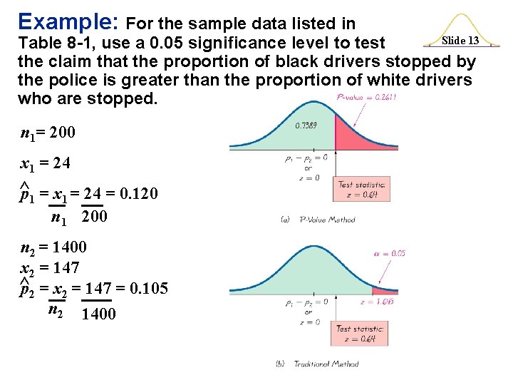
Example: For the sample data listed in Slide 9 Table 8 -1, use a 0. 05 significance level to test the claim that the proportion of black drivers stopped by the police is greater than the proportion of white drivers who are stopped. (p. 441)

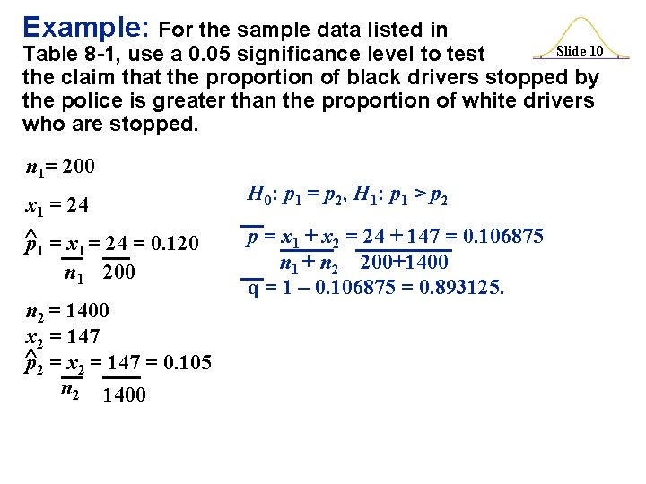
Example: For the sample data listed in Slide 10 Table 8 -1, use a 0. 05 significance level to test the claim that the proportion of black drivers stopped by the police is greater than the proportion of white drivers who are stopped. n 1= 200 x 1 = 24 ^p 1 = x 1 = 24 = 0. 120 n 1 200 n 2 = 1400 x 2 = 147 ^p 2 = x 2 = 147 = 0. 105 n 2 1400 H 0: p 1 = p 2, H 1: p 1 > p 2 p = x 1 + x 2 = 24 + 147 = 0. 106875 n 1 + n 2 200+1400 q = 1 – 0. 106875 = 0. 893125.

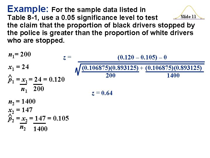
Example: For the sample data listed in Slide 11 Table 8 -1, use a 0. 05 significance level to test the claim that the proportion of black drivers stopped by the police is greater than the proportion of white drivers who are stopped. n 1= 200 z= x 1 = 24 ^p 1 = x 1 = 24 = 0. 120 n 1 200 n 2 = 1400 x 2 = 147 ^p 2 = x 2 = 147 = 0. 105 n 2 1400 (0. 120 – 0. 105) – 0 (0. 106875)(0. 893125) + (0. 106875)(0. 893125) 200 1400 z = 0. 64

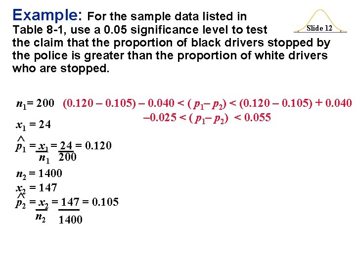
Example: For the sample data listed in Slide 12 Table 8 -1, use a 0. 05 significance level to test the claim that the proportion of black drivers stopped by the police is greater than the proportion of white drivers who are stopped. n 1= 200 (0. 120 – 0. 105) – 0. 040 < ( p 1– p 2) < (0. 120 – 0. 105) + 0. 040 – 0. 025 < ( p 1– p 2) < 0. 055 x 1 = 24 ^ p 1 = x 1 = 24 = 0. 120 n 1 200 n 2 = 1400 x 2 = 147 ^ p 2 = x 2 = 147 = 0. 105 n 2 1400

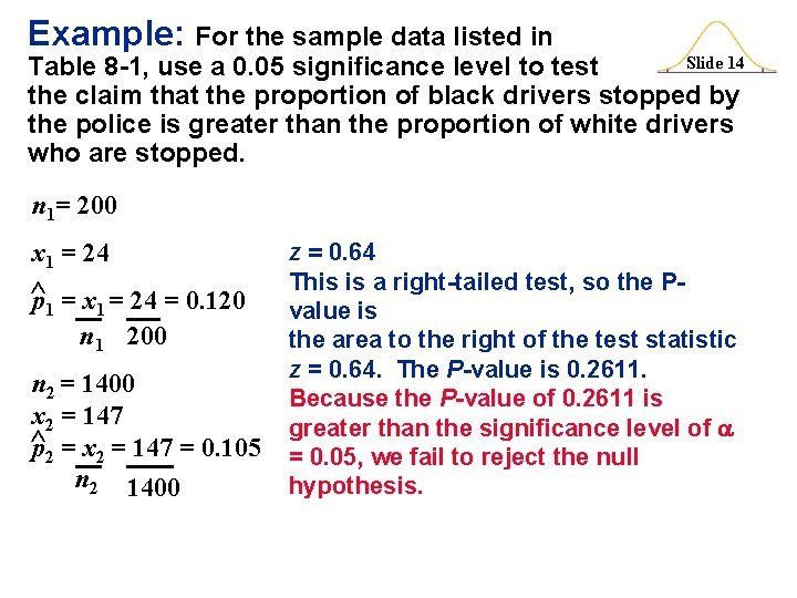
Example: For the sample data listed in Slide 13 Table 8 -1, use a 0. 05 significance level to test the claim that the proportion of black drivers stopped by the police is greater than the proportion of white drivers who are stopped. n 1= 200 x 1 = 24 ^p 1 = x 1 = 24 = 0. 120 n 1 200 n 2 = 1400 x 2 = 147 ^p 2 = x 2 = 147 = 0. 105 n 2 1400

Example: For the sample data listed in Slide 14 Table 8 -1, use a 0. 05 significance level to test the claim that the proportion of black drivers stopped by the police is greater than the proportion of white drivers who are stopped. n 1= 200 x 1 = 24 ^p 1 = x 1 = 24 = 0. 120 n 1 200 n 2 = 1400 x 2 = 147 ^p 2 = x 2 = 147 = 0. 105 n 2 1400 z = 0. 64 This is a right-tailed test, so the Pvalue is the area to the right of the test statistic z = 0. 64. The P-value is 0. 2611. Because the P-value of 0. 2611 is greater than the significance level of = 0. 05, we fail to reject the null hypothesis.

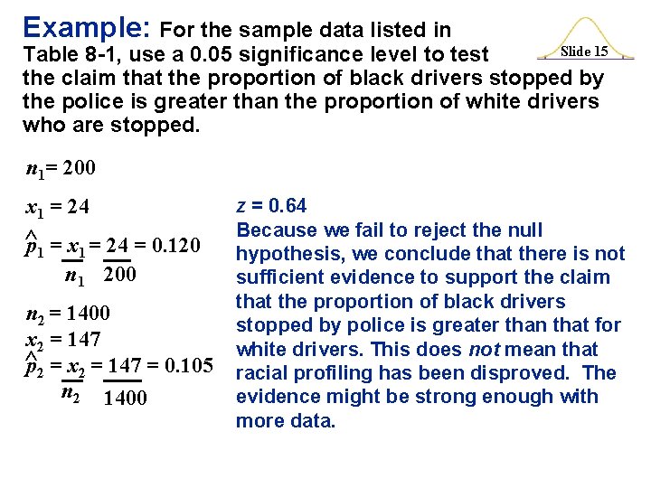
Example: For the sample data listed in Slide 15 Table 8 -1, use a 0. 05 significance level to test the claim that the proportion of black drivers stopped by the police is greater than the proportion of white drivers who are stopped. n 1= 200 x 1 = 24 ^p 1 = x 1 = 24 = 0. 120 n 1 200 n 2 = 1400 x 2 = 147 ^p 2 = x 2 = 147 = 0. 105 n 2 1400 z = 0. 64 Because we fail to reject the null hypothesis, we conclude that there is not sufficient evidence to support the claim that the proportion of black drivers stopped by police is greater than that for white drivers. This does not mean that racial profiling has been disproved. The evidence might be strong enough with more data.

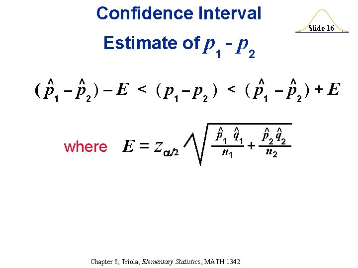
Confidence Interval Estimate of p 1 - p 2 ( p^1 – p^2 ) – E < ( p 1 – p 2 ) < ( p^1 where E = z Slide 16 – p^2 ) + ^ q^ p 1 1 2 2 n 1 + n 2 Chapter 8, Triola, Elementary Statistics, MATH 1342 E

Example: For the sample data listed in Slide 17 Table 8 -1, find a 90% confidence interval estimate of the difference between the two population proportions. (p. 444) n 1= 200 x 1 = 24 E = z ^ p 1 = x 1 = 24 = 0. 120 E = 1. 645 n 1 200 n 2 = 1400 x 2 = 147 ^ p 2 = x 2 = 147 = 0. 105 n 2 1400 E = 0. 400 ^ q^ p 1 1 2 2 n 1 + n 2 (. 12)(. 88)+(0. 105)(0. 895) 200 1400

Slide 18 Section 8 -3 Inferences about Two Means: Independent Samples Created by Erin Hodgess, Houston, Texas

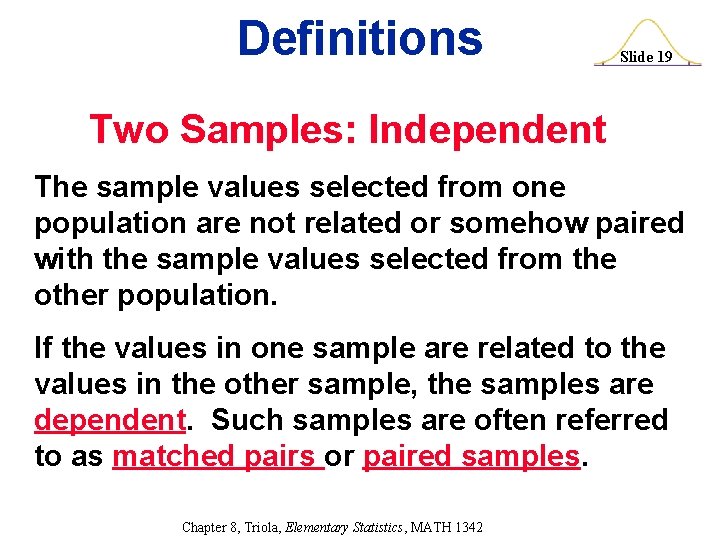
Definitions Slide 19 Two Samples: Independent The sample values selected from one population are not related or somehow paired with the sample values selected from the other population. If the values in one sample are related to the values in the other sample, the samples are dependent. Such samples are often referred to as matched pairs or paired samples. Chapter 8, Triola, Elementary Statistics, MATH 1342

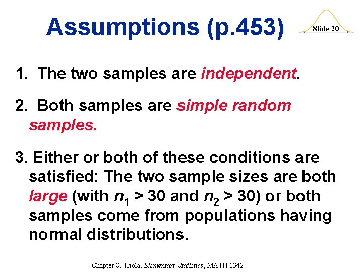
Assumptions (p. 453) Slide 20 1. The two samples are independent. 2. Both samples are simple random samples. 3. Either or both of these conditions are satisfied: The two sample sizes are both large (with n 1 > 30 and n 2 > 30) or both samples come from populations having normal distributions. Chapter 8, Triola, Elementary Statistics, MATH 1342

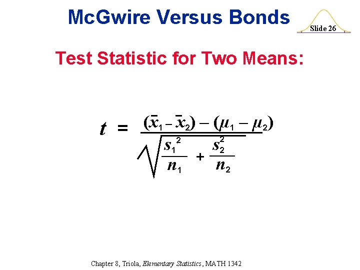
Hypothesis Test Statistic for Two Means: t (x 1 – x 2) – (µ 1 – µ 2) = 2. 2 s s 1 2 + n 2 n 1 Chapter 8, Triola, Elementary Statistics, MATH 1342 Slide 21

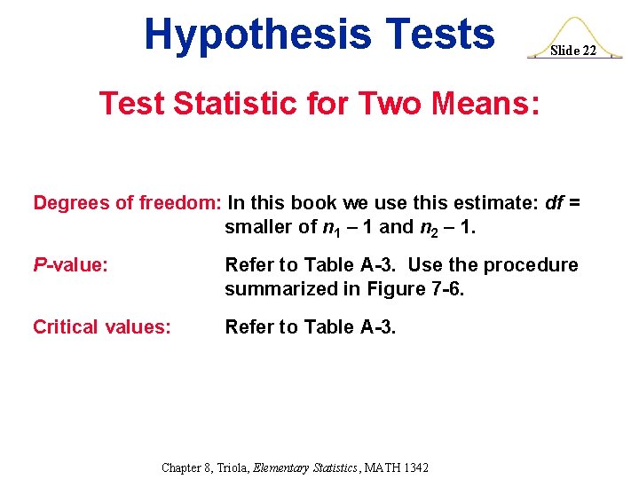
Hypothesis Tests Slide 22 Test Statistic for Two Means: Degrees of freedom: In this book we use this estimate: df = smaller of n 1 – 1 and n 2 – 1. P-value: Refer to Table A-3. Use the procedure summarized in Figure 7 -6. Critical values: Refer to Table A-3. Chapter 8, Triola, Elementary Statistics, MATH 1342

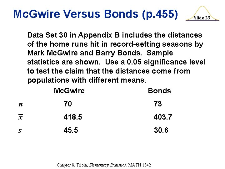
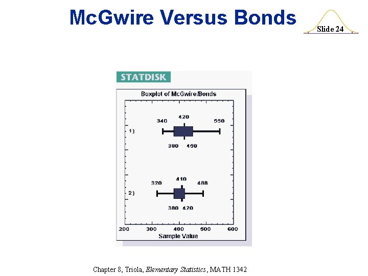
Mc. Gwire Versus Bonds (p. 455) Slide 23 Data Set 30 in Appendix B includes the distances of the home runs hit in record-setting seasons by Mark Mc. Gwire and Barry Bonds. Sample statistics are shown. Use a 0. 05 significance level to test the claim that the distances come from populations with different means. Mc. Gwire Bonds n 70 73 x 418. 5 403. 7 s 45. 5 30. 6 Chapter 8, Triola, Elementary Statistics, MATH 1342

Mc. Gwire Versus Bonds Chapter 8, Triola, Elementary Statistics, MATH 1342 Slide 24

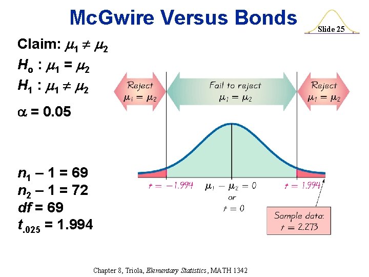
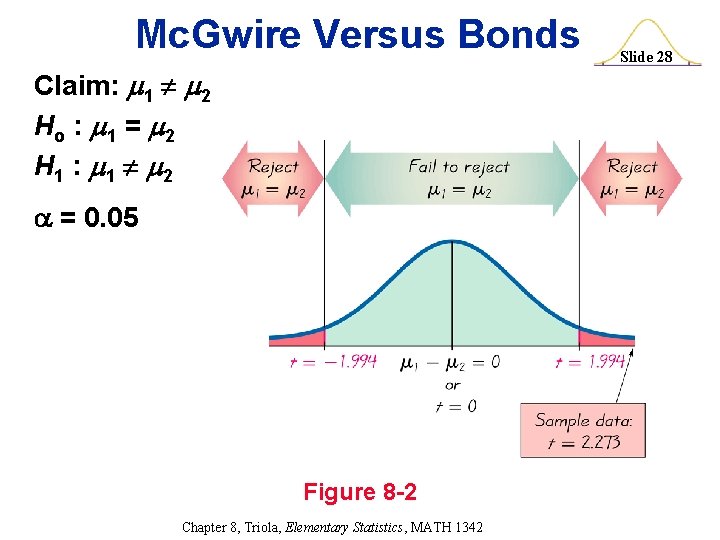
Mc. Gwire Versus Bonds Claim: 1 2 Ho : 1 = 2 H 1 : 1 2 = 0. 05 n 1 – 1 = 69 n 2 – 1 = 72 df = 69 t. 025 = 1. 994 Chapter 8, Triola, Elementary Statistics, MATH 1342 Slide 25

Mc. Gwire Versus Bonds Test Statistic for Two Means: t (x 1 – x 2) – (µ 1 – µ 2) = 2. 2 s 1 s 2 + n 2 n 1 Chapter 8, Triola, Elementary Statistics, MATH 1342 Slide 26

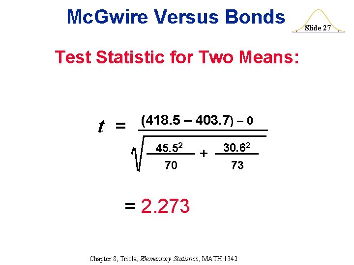
Mc. Gwire Versus Bonds Test Statistic for Two Means: t = (418. 5 – 403. 7) – 0 45. 52 70 + 30. 62 73 = 2. 273 Chapter 8, Triola, Elementary Statistics, MATH 1342 Slide 27

Mc. Gwire Versus Bonds Claim: 1 2 Ho : 1 = 2 H 1 : 1 2 = 0. 05 Figure 8 -2 Chapter 8, Triola, Elementary Statistics, MATH 1342 Slide 28

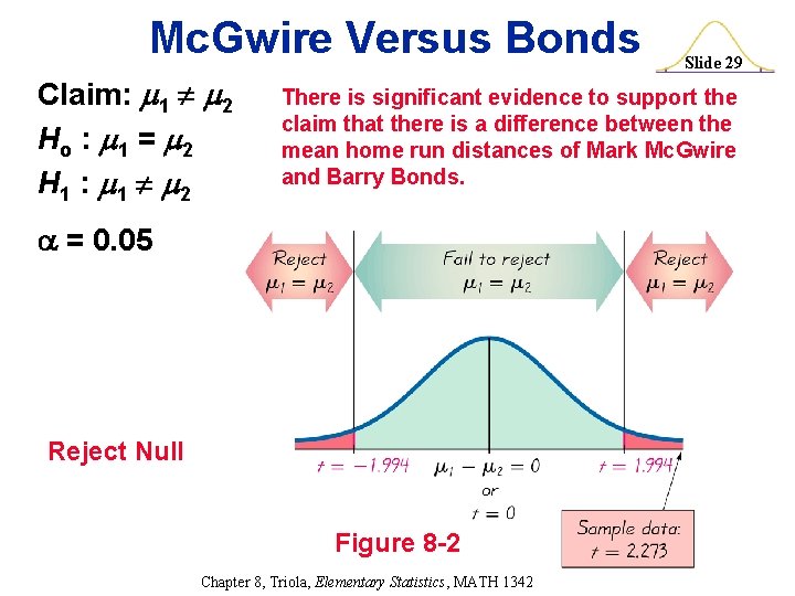
Mc. Gwire Versus Bonds Claim: 1 2 Ho : 1 = 2 H 1 : 1 2 Slide 29 There is significant evidence to support the claim that there is a difference between the mean home run distances of Mark Mc. Gwire and Barry Bonds. = 0. 05 Reject Null Figure 8 -2 Chapter 8, Triola, Elementary Statistics, MATH 1342

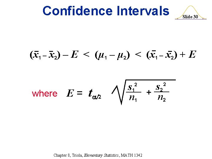
Confidence Intervals Slide 30 (x 1 – x 2) – E < (µ 1 – µ 2) < (x 1 – x 2) + E where E = t s 2 s + n 2 n 1 2 1 Chapter 8, Triola, Elementary Statistics, MATH 1342 2

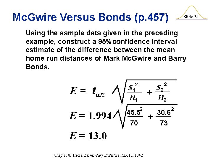
Mc. Gwire Versus Bonds (p. 457) Slide 31 Using the sample data given in the preceding example, construct a 95%confidence interval estimate of the difference between the mean home run distances of Mark Mc. Gwire and Barry Bonds. E = t E = 1. 994 s 2 s + n 2 n 1 2 2 1 2 45. 5 70 E = 13. 0 Chapter 8, Triola, Elementary Statistics, MATH 1342 + 30. 6 73 2

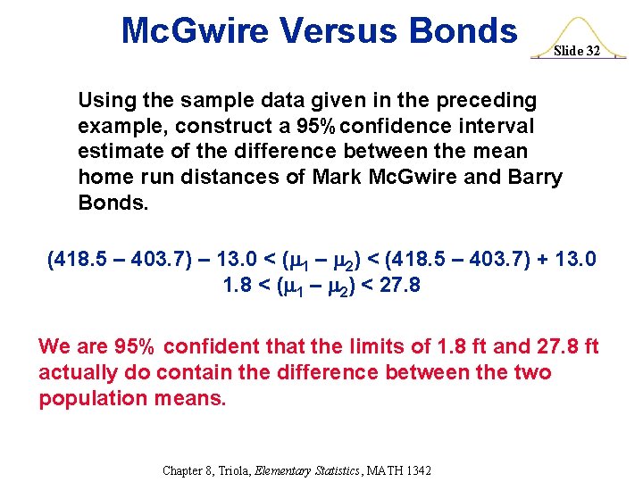
Mc. Gwire Versus Bonds Slide 32 Using the sample data given in the preceding example, construct a 95%confidence interval estimate of the difference between the mean home run distances of Mark Mc. Gwire and Barry Bonds. (418. 5 – 403. 7) – 13. 0 < ( 1 – 2) < (418. 5 – 403. 7) + 13. 0 1. 8 < ( 1 – 2) < 27. 8 We are 95% confident that the limits of 1. 8 ft and 27. 8 ft actually do contain the difference between the two population means. Chapter 8, Triola, Elementary Statistics, MATH 1342

Slide 33 Section 8 -4 Inferences from Matched Pairs Created by Erin Hodgess, Houston, Texas

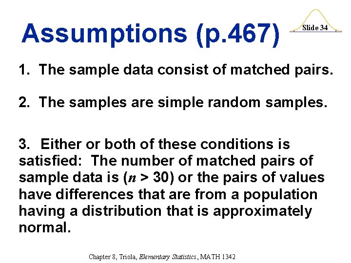
Assumptions (p. 467) Slide 34 1. The sample data consist of matched pairs. 2. The samples are simple random samples. 3. Either or both of these conditions is satisfied: The number of matched pairs of sample data is (n > 30) or the pairs of values have differences that are from a population having a distribution that is approximately normal. Chapter 8, Triola, Elementary Statistics, MATH 1342

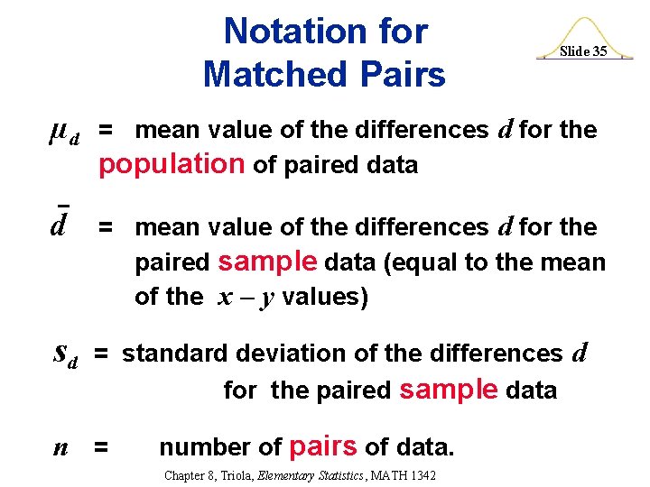
Notation for Matched Pairs Slide 35 µd = mean value of the differences d for the population of paired data d = mean value of the differences d for the paired sample data (equal to the mean of the x – y values) sd = standard deviation of the differences d for the paired sample data n = number of pairs of data. Chapter 8, Triola, Elementary Statistics, MATH 1342

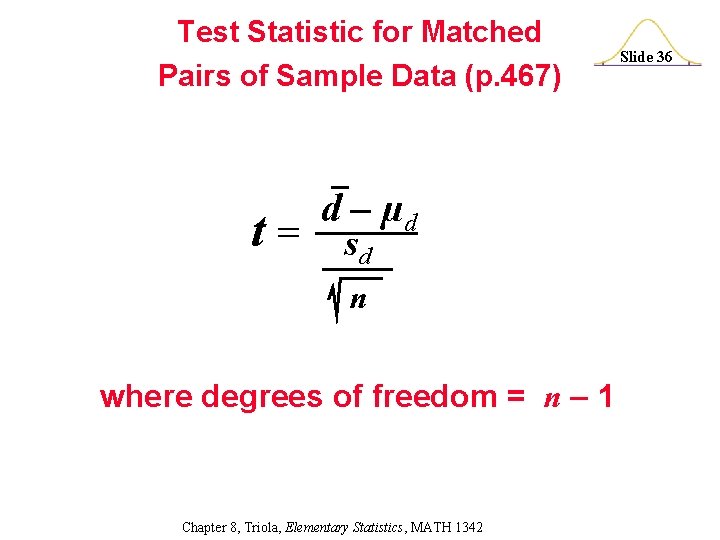
Test Statistic for Matched Pairs of Sample Data (p. 467) t= d – µd sd n where degrees of freedom = n – 1 Chapter 8, Triola, Elementary Statistics, MATH 1342 Slide 36

P-values and Critical Values Slide 37 Use Table A-3 (t-distribution) on p. 736. Chapter 8, Triola, Elementary Statistics, MATH 1342

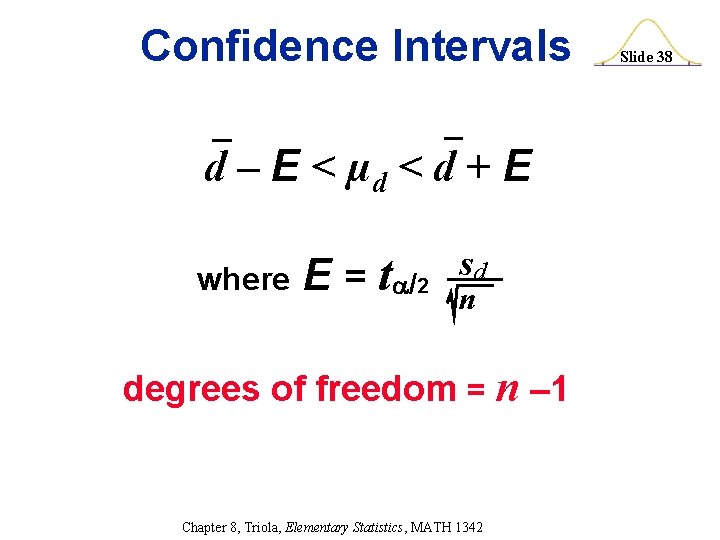
Confidence Intervals d – E < µd < d + E where E = t /2 sd n degrees of freedom = n – 1 Chapter 8, Triola, Elementary Statistics, MATH 1342 Slide 38

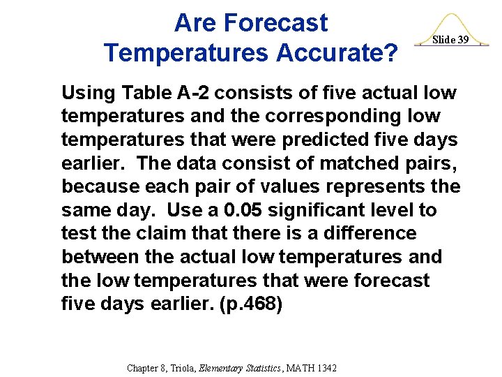
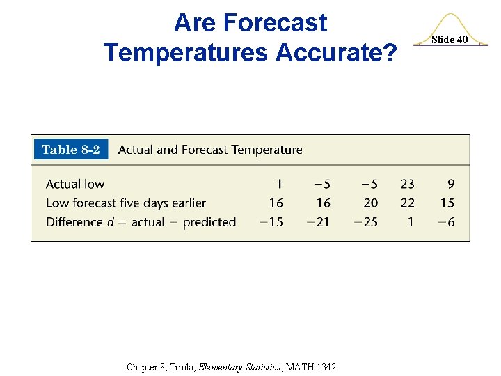
Are Forecast Temperatures Accurate? Slide 39 Using Table A-2 consists of five actual low temperatures and the corresponding low temperatures that were predicted five days earlier. The data consist of matched pairs, because each pair of values represents the same day. Use a 0. 05 significant level to test the claim that there is a difference between the actual low temperatures and the low temperatures that were forecast five days earlier. (p. 468) Chapter 8, Triola, Elementary Statistics, MATH 1342

Are Forecast Temperatures Accurate? Chapter 8, Triola, Elementary Statistics, MATH 1342 Slide 40

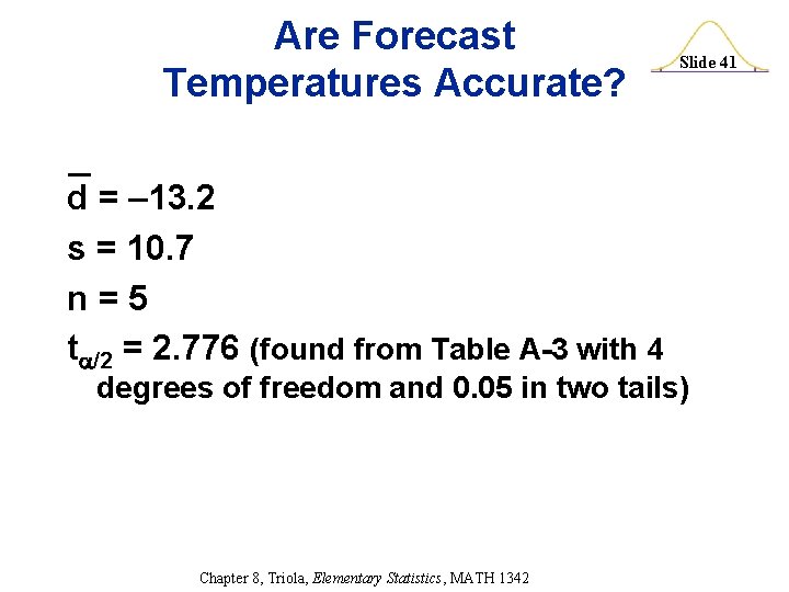
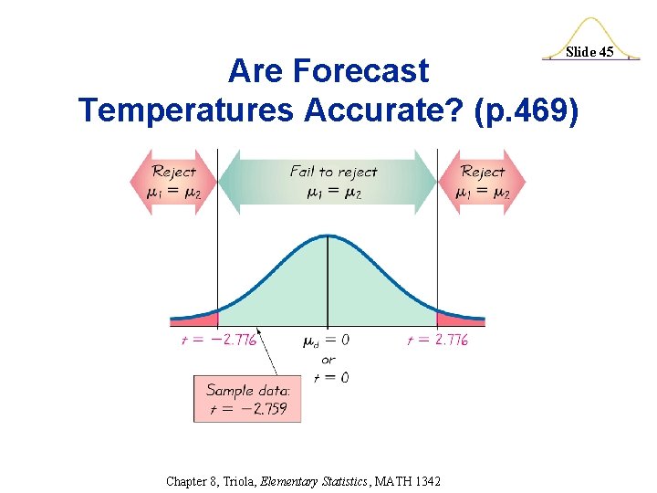
Are Forecast Temperatures Accurate? d = – 13. 2 s = 10. 7 n=5 t /2 = 2. 776 (found from Table A-3 with 4 Slide 41 degrees of freedom and 0. 05 in two tails) Chapter 8, Triola, Elementary Statistics, MATH 1342

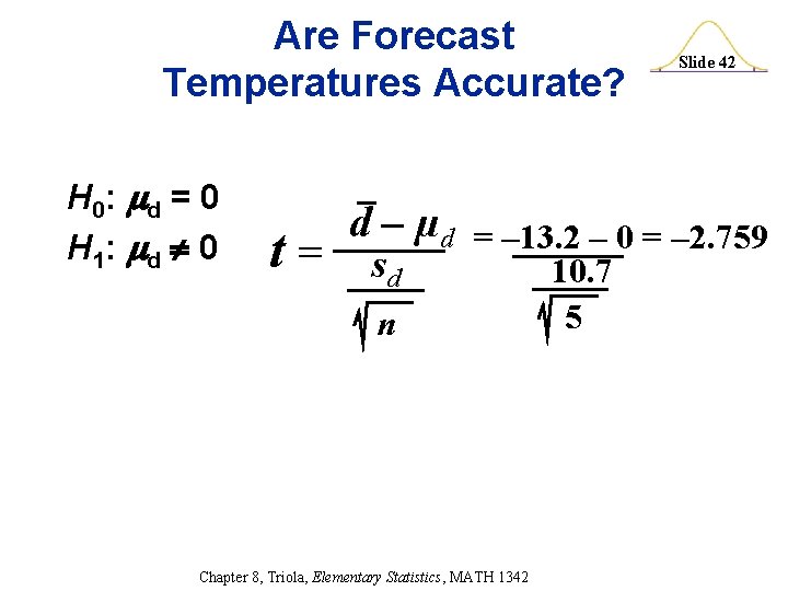
Are Forecast Temperatures Accurate? H 0: d = 0 H 1: d 0 t= d – µd sd n Slide 42 = – 13. 2 – 0 = – 2. 759 10. 7 5 Chapter 8, Triola, Elementary Statistics, MATH 1342

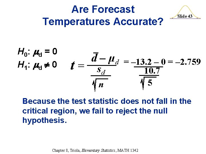
Are Forecast Temperatures Accurate? H 0: d = 0 H 1: d 0 t= d – µd sd n Slide 43 = – 13. 2 – 0 = – 2. 759 10. 7 5 Because the test statistic does not fall in the critical region, we fail to reject the null hypothesis. Chapter 8, Triola, Elementary Statistics, MATH 1342

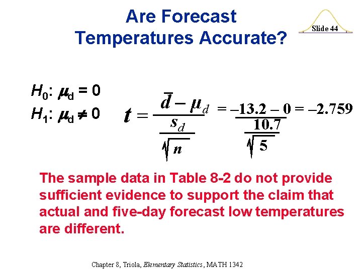
Are Forecast Temperatures Accurate? H 0: d = 0 H 1: d 0 t= d – µd sd n Slide 44 = – 13. 2 – 0 = – 2. 759 10. 7 5 The sample data in Table 8 -2 do not provide sufficient evidence to support the claim that actual and five-day forecast low temperatures are different. Chapter 8, Triola, Elementary Statistics, MATH 1342

Slide 45 Are Forecast Temperatures Accurate? (p. 469) Chapter 8, Triola, Elementary Statistics, MATH 1342

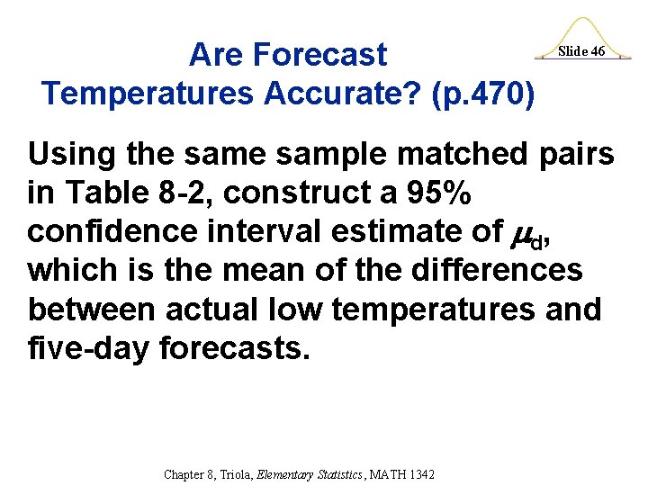
Are Forecast Temperatures Accurate? (p. 470) Slide 46 Using the sample matched pairs in Table 8 -2, construct a 95% confidence interval estimate of d, which is the mean of the differences between actual low temperatures and five-day forecasts. Chapter 8, Triola, Elementary Statistics, MATH 1342

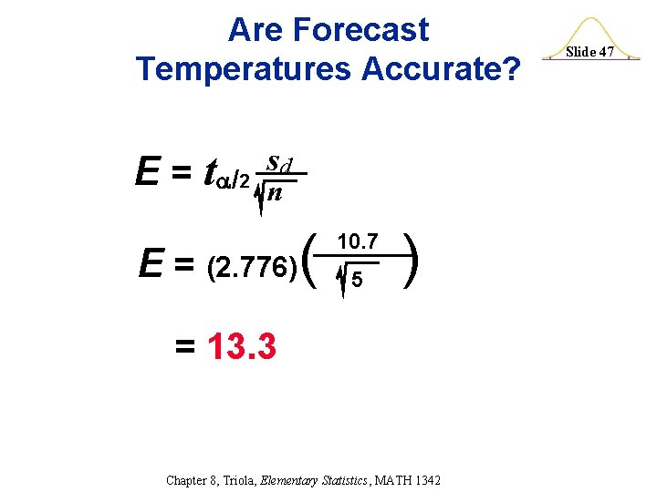
Are Forecast Temperatures Accurate? E = t /2 sd n E = (2. 776)( 10. 7 5 ) = 13. 3 Chapter 8, Triola, Elementary Statistics, MATH 1342 Slide 47

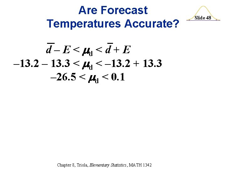
Are Forecast Temperatures Accurate? d – E < d + E – 13. 2 – 13. 3 < d < – 13. 2 + 13. 3 – 26. 5 < d < 0. 1 Chapter 8, Triola, Elementary Statistics, MATH 1342 Slide 48

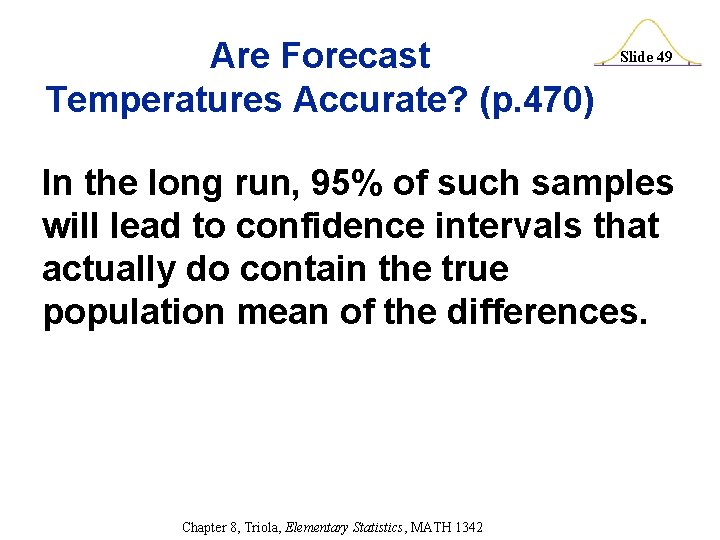
Are Forecast Temperatures Accurate? (p. 470) Slide 49 In the long run, 95% of such samples will lead to confidence intervals that actually do contain the true population mean of the differences. Chapter 8, Triola, Elementary Statistics, MATH 1342

Slide 50 Section 8 -5 Comparing Variation in Two Samples Created by Erin Hodgess, Houston, Texas

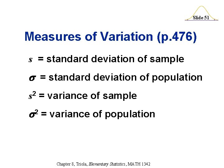
Slide 51 Measures of Variation (p. 476) s = standard deviation of sample = standard deviation of population s 2 = variance of sample 2 = variance of population Chapter 8, Triola, Elementary Statistics, MATH 1342

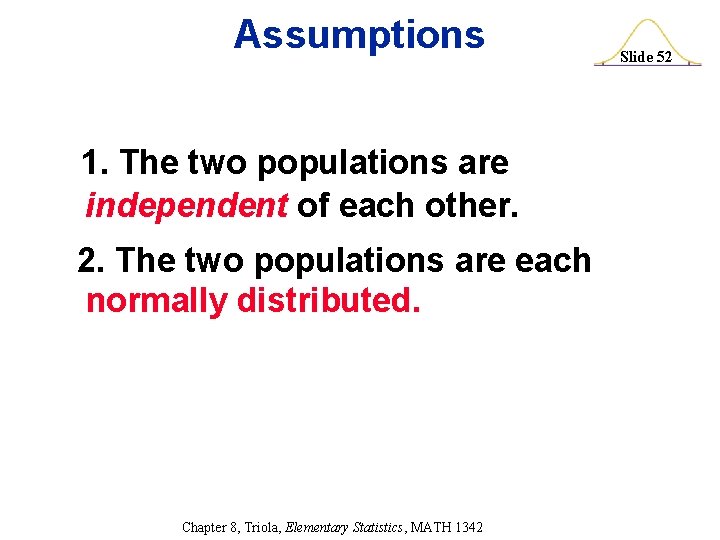
Assumptions 1. The two populations are independent of each other. 2. The two populations are each normally distributed. Chapter 8, Triola, Elementary Statistics, MATH 1342 Slide 52

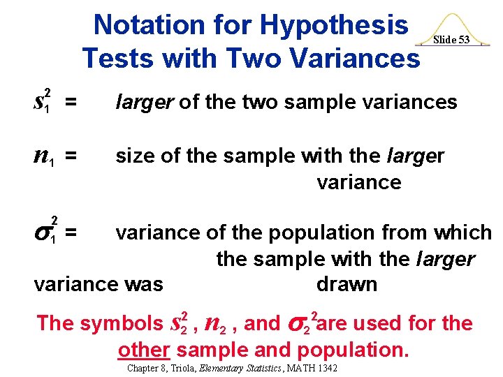
Notation for Hypothesis Tests with Two Variances s 2 Slide 53 1 = larger of the two sample variances n = size of the sample with the larger variance 1 2 variance of the population from which the sample with the larger variance was drawn 1 = The symbols s 2 , n 2 , and 2 are used for the other sample and population. 2 2 Chapter 8, Triola, Elementary Statistics, MATH 1342

Test Statistic for Hypothesis Tests with Two Variances F= s s Slide 54 2 1 2 2 Critical Values: Using Table A-5, we obtain critical F values that are determined by the following three values: 1. The significance level . 2. Numerator degrees of freedom (df 1) = n 1 – 1 3. Denominator degrees of freedom (df 2) = n 2 – 1 Chapter 8, Triola, Elementary Statistics, MATH 1342

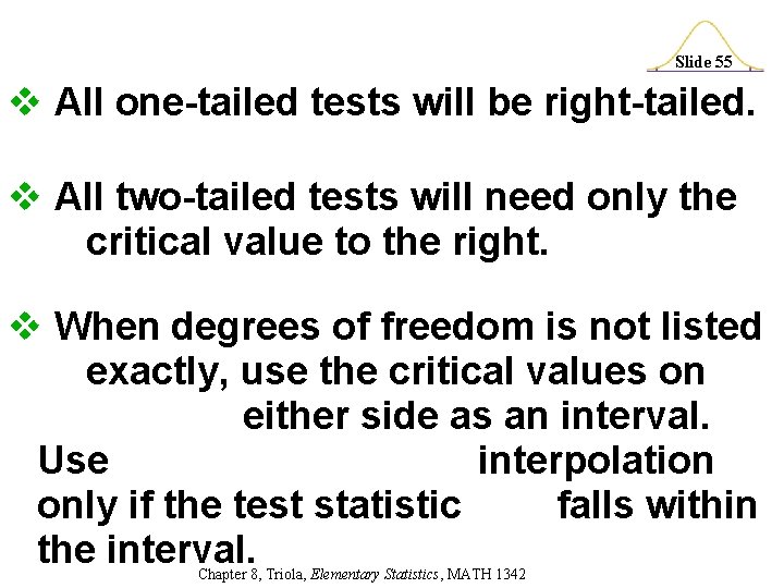
Slide 55 v All one-tailed tests will be right-tailed. v All two-tailed tests will need only the critical value to the right. v When degrees of freedom is not listed exactly, use the critical values on either side as an interval. Use interpolation only if the test statistic falls within the interval. Chapter 8, Triola, Elementary Statistics, MATH 1342

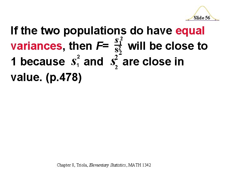
Slide 56 If the two populations do have equal s 12 variances, then F= s 22 will be close to 2 2 1 because s 1 and s 2 are close in value. (p. 478) Chapter 8, Triola, Elementary Statistics, MATH 1342

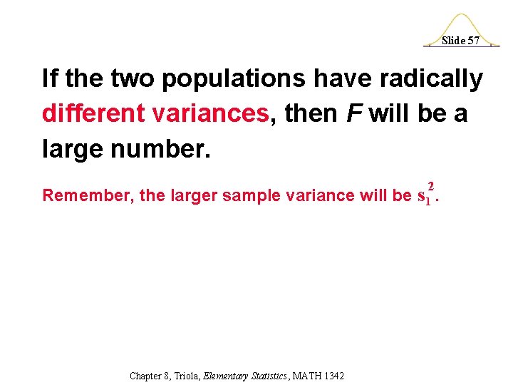
Slide 57 If the two populations have radically different variances, then F will be a large number. 2 Remember, the larger sample variance will be s 1. Chapter 8, Triola, Elementary Statistics, MATH 1342

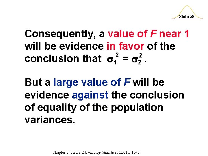
Slide 58 Consequently, a value of F near 1 will be evidence in favor of the 2 2 conclusion that 1 = 2. But a large value of F will be evidence against the conclusion of equality of the population variances. Chapter 8, Triola, Elementary Statistics, MATH 1342

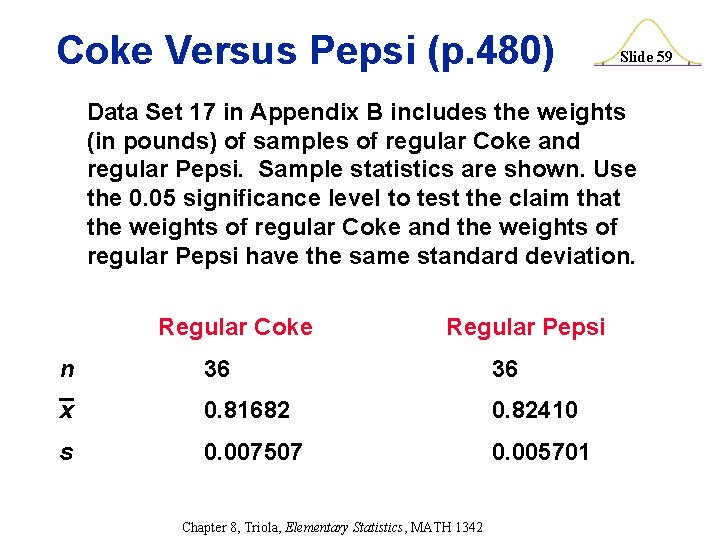
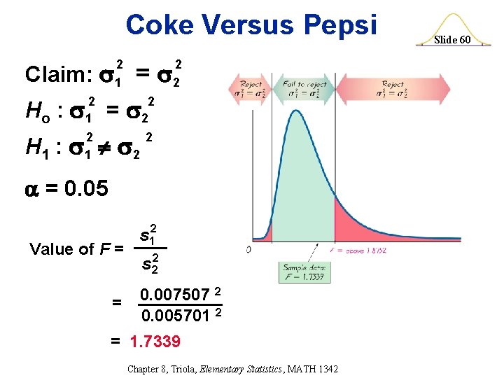
Coke Versus Pepsi (p. 480) Slide 59 Data Set 17 in Appendix B includes the weights (in pounds) of samples of regular Coke and regular Pepsi. Sample statistics are shown. Use the 0. 05 significance level to test the claim that the weights of regular Coke and the weights of regular Pepsi have the same standard deviation. Regular Coke Regular Pepsi n 36 36 x 0. 81682 0. 82410 s 0. 007507 0. 005701 Chapter 8, Triola, Elementary Statistics, MATH 1342

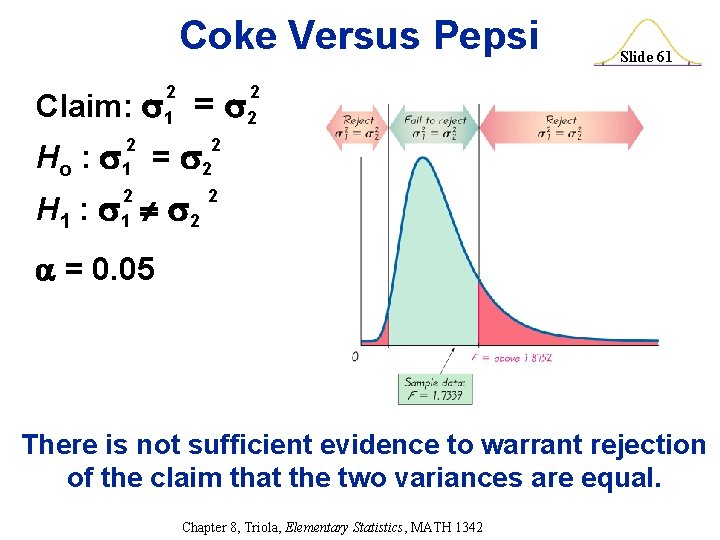
Coke Versus Pepsi Claim: = 2 1 Ho : = 2 1 H 1 : 2 2 2 = 0. 05 Value of F = = s 12 s 22 0. 007507 2 0. 005701 2 = 1. 7339 Chapter 8, Triola, Elementary Statistics, MATH 1342 Slide 60

Coke Versus Pepsi Claim: = 2 1 Ho : = 2 1 H 1 : 2 Slide 61 2 2 2 = 0. 05 There is not sufficient evidence to warrant rejection of the claim that the two variances are equal. Chapter 8, Triola, Elementary Statistics, MATH 1342