Chapter 8 Forecasting 1 Operations Management 6 th

Learning Objectives 2 Identify principles of forecasting. Explain the steps involved in the forecasting

Learning Objectives - cont'd 3 Describe causal modeling using linear regression. Compute forecast accuracy.

Forecasting - Defined 4 Predicting future events One of the most important business functions

Principles of Forecasting 5 Many types of forecasting models differ in complexity and amount

Steps in the Forecasting Process 6 Decide what needs to be forecast Level of

Types of Forecasting Methods – cont’d 7 Classified into two groups: Copyright © 2016

Types of Forecasting Models 8 Qualitative methods – judgmental methods Forecasts generated subjectively by

Qualitative Methods 9 Copyright © 2016 John Wiley & Sons, Inc.

Quantitative Methods 10 Time Series Models: Assumes information needed to generate a forecast is

Time Series Models 11 Forecaster looks for data patterns as Data = historic pattern

Time Series Patterns 12 Copyright © 2016 John Wiley & Sons, Inc.

Time Series Models 13 Naive: The forecast is equal to the actual value observed

Time Series Models cont'd 14 Exponential Smoothing: Most frequently used time series method because

Time Series Problem 15 Determine forecast for periods 7 & 8 2 -period moving

Time Series Problem 16 Let us use the following formulas for the 2 -period

Time Series Problem Solution 17 Period Actual 1 300 2 315 3 290 307.

Time Series Problem 18 Now we use the formulas for the 4 - period

Time Series Problem Solution 19 Period Actual 1 300 2 315 3 290 4

Time Series Problem 20 Determine forecast for periods 7 & 8 Exponential smoothing with

Time Series Problem Solution 21 ES a=0. 2 F 6=375 Period Actual 1 300

Time Series Problem 22 Determine forecast for periods 7 & 8 Exponential smoothing with

Time Series Problem Solution 23 Period Actual ES a=0. 2 F 1=300 1 300

Linear Trend Line 24 A time series technique that computes a forecast with trend

Causal Models 25 Often, leading indicators can help to predict changes in future demand

Linear Regression 26 Identify dependent (y) and independent (x) variables Solve for the slope

Linear Regression Problem: A maker of golf shirts has been tracking the relationship between

Correlation Coefficient- How Good is the Fit? 29 Correlation coefficient (r) measures the direction

Measuring Forecast Accuracy 30 Forecasts are never perfect Need to measure over time Need

Measuring Forecasting Accuracy 31 Mean Absolute Deviation (MAD) measures the total error in a

Mean Absolute Deviation 32 |At - Ft| Period Actual 1 300 -- 2 315

Selecting the Right Forecasting Model 33 The amount & type of available data 1.

Forecasting Software 34 Spreadsheets Microsoft Excel, Quattro Pro, Lotus 1 -2 -3 Limited statistical

Forecasting Within OM: How It All Fits Together 35 Forecasts impact not only other

Forecasting within OM - cont'd 36 Forecasts drive strategic operations decisions, such as: Choice

Forecasting Across the Organization 37 Forecasting is critical to management of all organizational functional

Chapter 8 Highlights 38 Three basic principles of forecasting are: forecasts are rarely perfect,

Chapter 8 Highlights - cont'd 39 Time series models are based on the assumption

Chapter 8 Highlights - cont'd 40 A simple causal model is linear regression in

Slides: 40

Download presentation

Learning Objectives 2 Identify principles of forecasting. Explain the steps involved in the forecasting process. Identify types of forecasting methods and their characteristics. Describe time series models. Copyright © 2016 John Wiley & Sons, Inc.

Learning Objectives - cont'd 3 Describe causal modeling using linear regression. Compute forecast accuracy. Explain the factors that should be considered when selecting a forecasting model. Explain the nine-step process of CPFR. Copyright © 2016 John Wiley & Sons, Inc.

Forecasting - Defined 4 Predicting future events One of the most important business functions as decisions are based on a forecast of the future Goal: Generate good forecasts on the average over time and keep errors low Forecasting is an ongoing process Copyright © 2016 John Wiley & Sons, Inc.

Principles of Forecasting 5 Many types of forecasting models differ in complexity and amount of data & way they generate forecasts. Common features include: 1. Forecasts are rarely perfect 2. Forecasts are more accurate for grouped data than for individual items 3. Forecast are more accurate for shorter than longer time periods Copyright © 2016 John Wiley & Sons, Inc.

Steps in the Forecasting Process 6 Decide what needs to be forecast Level of detail, units of analysis & time horizon required Evaluate and analyze appropriate data Identify needed data & whether it’s available Select and test the forecasting model Cost, ease of use & accuracy Generate the forecast Monitor forecast accuracy over time Copyright © 2016 John Wiley & Sons, Inc.

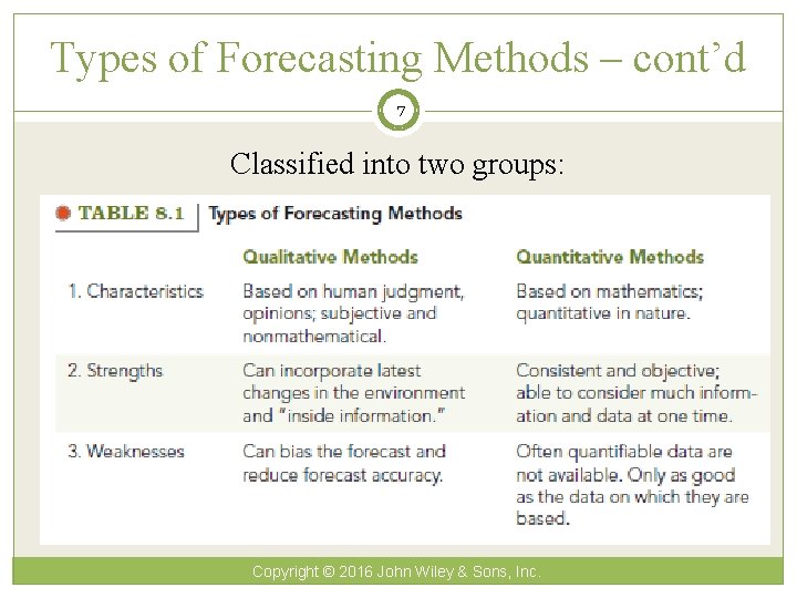
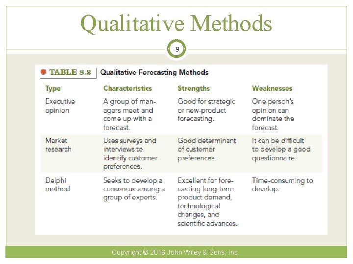
Types of Forecasting Models 8 Qualitative methods – judgmental methods Forecasts generated subjectively by the forecaster Educated guesses Quantitative methods – based on mathematical modeling: Forecasts generated through mathematical modeling Copyright © 2016 John Wiley & Sons, Inc.

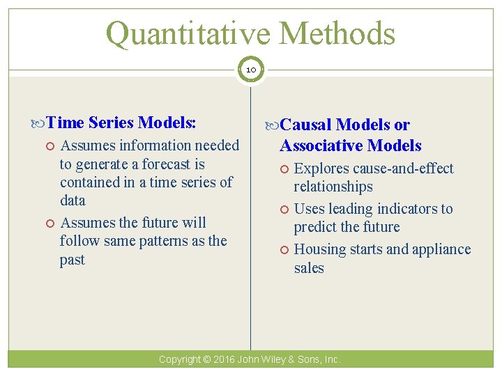
Quantitative Methods 10 Time Series Models: Assumes information needed to generate a forecast is contained in a time series of data Assumes the future will follow same patterns as the past Causal Models or Associative Models Explores cause-and-effect relationships Uses leading indicators to predict the future Housing starts and appliance sales Copyright © 2016 John Wiley & Sons, Inc.

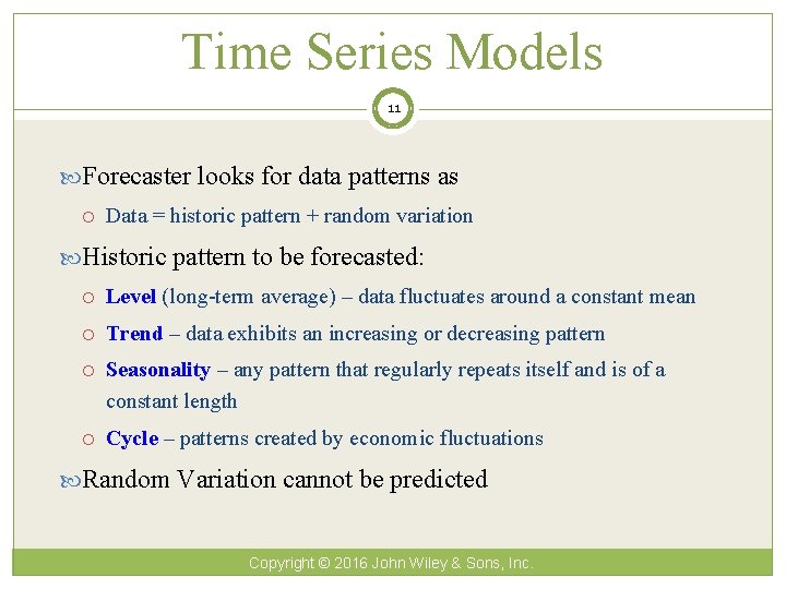
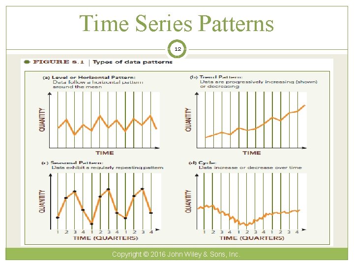
Time Series Models 11 Forecaster looks for data patterns as Data = historic pattern + random variation Historic pattern to be forecasted: Level (long-term average) – data fluctuates around a constant mean Trend – data exhibits an increasing or decreasing pattern Seasonality – any pattern that regularly repeats itself and is of a constant length Cycle – patterns created by economic fluctuations Random Variation cannot be predicted Copyright © 2016 John Wiley & Sons, Inc.

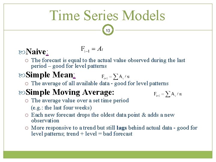
Time Series Models 13 Naive: The forecast is equal to the actual value observed during the last period – good for level patterns Simple Mean: The average of all available data - good for level patterns Simple Moving Average: The average value over a set time period (e. g. : the last four weeks) Each new forecast drops the oldest data point & adds a new observation More responsive to a trend but still lags behind actual data - good for level patterns; trend + level = bad forecast

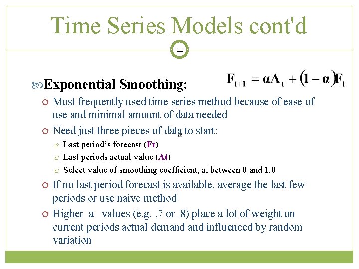
Time Series Models cont'd 14 Exponential Smoothing: Most frequently used time series method because of ease of use and minimal amount of data needed Need just three pieces of data to start: Last period’s forecast (Ft) Last periods actual value (At) Select value of smoothing coefficient, a, between 0 and 1. 0 If no last period forecast is available, average the last few periods or use naive method Higher a values (e. g. . 7 or. 8) place a lot of weight on current periods actual demand influenced by random variation

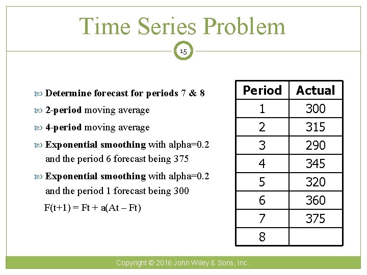
Time Series Problem 15 Determine forecast for periods 7 & 8 2 -period moving average 4 -period moving average Exponential smoothing with alpha=0. 2 Period 1 2 3 Actual 300 315 290 4 5 6 7 8 345 320 360 375 and the period 6 forecast being 375 Exponential smoothing with alpha=0. 2 and the period 1 forecast being 300 F(t+1) = Ft + a(At – Ft) Copyright © 2016 John Wiley & Sons, Inc.

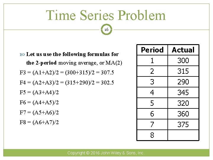
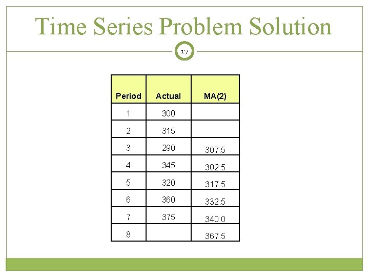
Time Series Problem 16 Let us use the following formulas for the 2 -period moving average, or MA(2) F 3 = (A 1+A 2)/2 = (300+315)/2 = 307. 5 F 4 = (A 2+A 3)/2 = (315+290)/2 = 302. 5 Period 1 2 3 Actual 300 315 290 4 5 6 7 8 345 320 360 375 F 5 = (A 3+A 4)/2 F 6 = (A 4+A 5)/2 F 7 = (A 5+A 6)/2 F 8 = (A 6+A 7)/2 Copyright © 2016 John Wiley & Sons, Inc.

Time Series Problem Solution 17 Period Actual 1 300 2 315 3 290 307. 5 4 345 302. 5 5 320 317. 5 6 360 332. 5 7 375 340. 0 8 MA(2) 367. 5

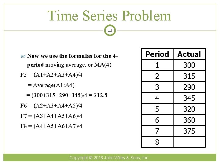
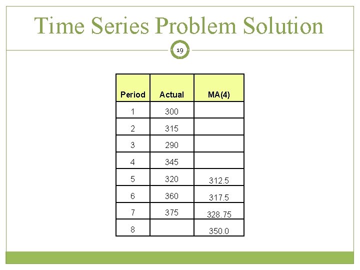
Time Series Problem 18 Now we use the formulas for the 4 - period moving average, or MA(4) F 5 = (A 1+A 2+A 3+A 4)/4 = Average(A 1: A 4) Period 1 2 3 Actual 300 315 290 4 5 6 7 8 345 320 360 375 = (300+315+290+345)/4 = 312. 5 F 6 = (A 2+A 3+A 4+A 5)/4 F 7 = (A 3+A 4+A 5+A 6)/4 F 8 = (A 4+A 5+A 6+A 7)/4 Copyright © 2016 John Wiley & Sons, Inc.

Time Series Problem Solution 19 Period Actual 1 300 2 315 3 290 4 345 5 320 312. 5 6 360 317. 5 7 375 328. 75 8 MA(4) 350. 0

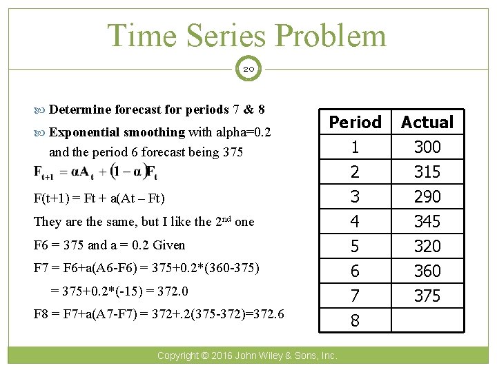
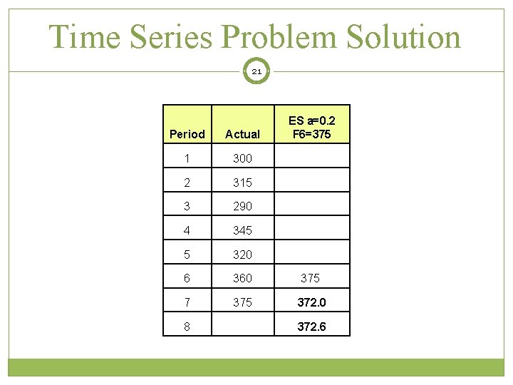
Time Series Problem 20 Determine forecast for periods 7 & 8 Exponential smoothing with alpha=0. 2 and the period 6 forecast being 375 F(t+1) = Ft + a(At – Ft) Period 1 2 3 Actual 300 315 290 4 5 6 7 8 345 320 360 375 They are the same, but I like the 2 nd one F 6 = 375 and a = 0. 2 Given F 7 = F 6+a(A 6 -F 6) = 375+0. 2*(360 -375) = 375+0. 2*(-15) = 372. 0 F 8 = F 7+a(A 7 -F 7) = 372+. 2(375 -372)=372. 6 Copyright © 2016 John Wiley & Sons, Inc.

Time Series Problem Solution 21 ES a=0. 2 F 6=375 Period Actual 1 300 2 315 3 290 4 345 5 320 6 360 375 7 375 372. 0 8 372. 6

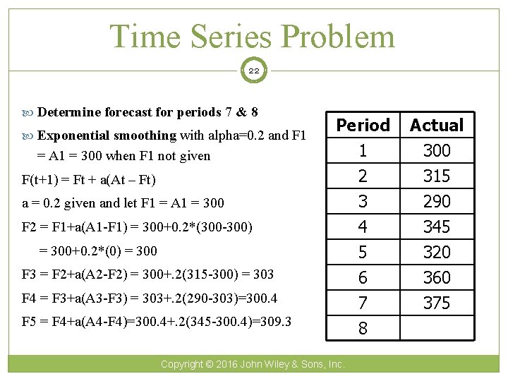
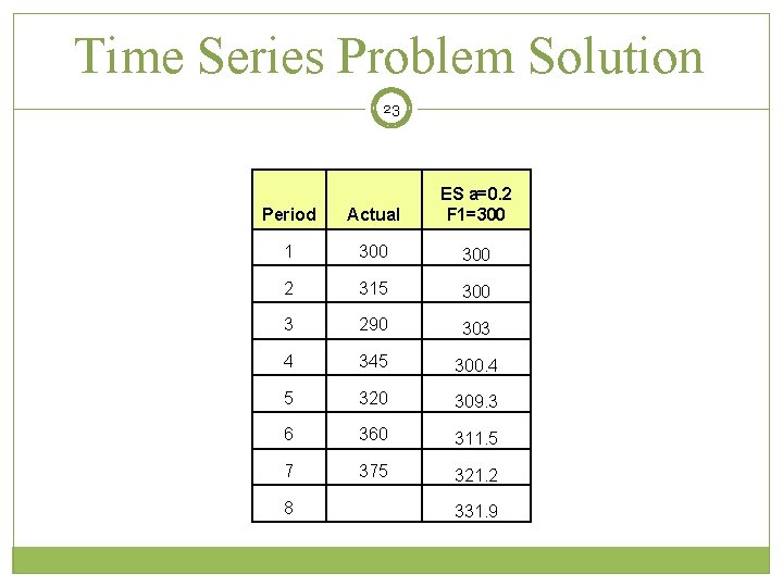
Time Series Problem 22 Determine forecast for periods 7 & 8 Exponential smoothing with alpha=0. 2 and F 1 = A 1 = 300 when F 1 not given F(t+1) = Ft + a(At – Ft) a = 0. 2 given and let F 1 = A 1 = 300 Period 1 2 3 Actual 300 315 290 4 5 6 7 8 345 320 360 375 F 2 = F 1+a(A 1 -F 1) = 300+0. 2*(300 -300) = 300+0. 2*(0) = 300 F 3 = F 2+a(A 2 -F 2) = 300+. 2(315 -300) = 303 F 4 = F 3+a(A 3 -F 3) = 303+. 2(290 -303)=300. 4 F 5 = F 4+a(A 4 -F 4)=300. 4+. 2(345 -300. 4)=309. 3 Copyright © 2016 John Wiley & Sons, Inc.

Time Series Problem Solution 23 Period Actual ES a=0. 2 F 1=300 1 300 2 315 300 3 290 303 4 345 300. 4 5 320 309. 3 6 360 311. 5 7 375 321. 2 8 331. 9

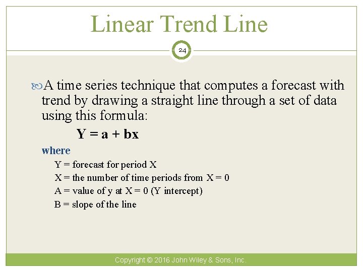
Linear Trend Line 24 A time series technique that computes a forecast with trend by drawing a straight line through a set of data using this formula: Y = a + bx where Y = forecast for period X X = the number of time periods from X = 0 A = value of y at X = 0 (Y intercept) B = slope of the line Copyright © 2016 John Wiley & Sons, Inc.

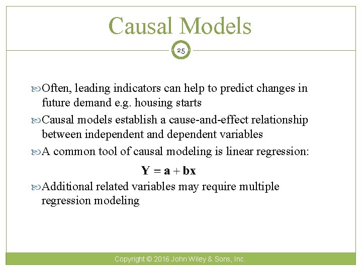
Causal Models 25 Often, leading indicators can help to predict changes in future demand e. g. housing starts Causal models establish a cause-and-effect relationship between independent and dependent variables A common tool of causal modeling is linear regression: Additional related variables may require multiple regression modeling Copyright © 2016 John Wiley & Sons, Inc.

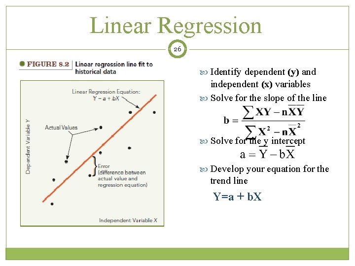
Linear Regression 26 Identify dependent (y) and independent (x) variables Solve for the slope of the line Solve for the y intercept Develop your equation for the trend line Y=a + b. X

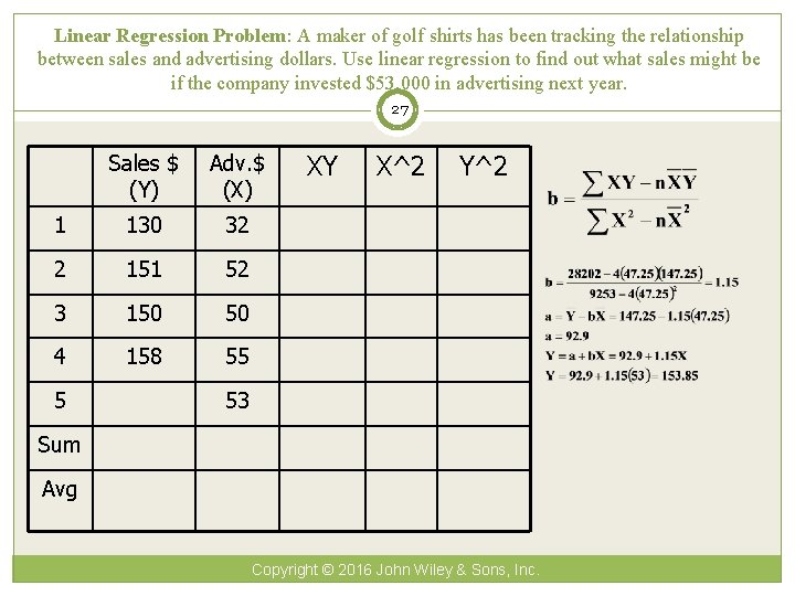
Linear Regression Problem: A maker of golf shirts has been tracking the relationship between sales and advertising dollars. Use linear regression to find out what sales might be if the company invested $53, 000 in advertising next year. 27 Sales $ (Y) Adv. $ (X) 1 130 32 2 151 52 3 150 50 4 158 55 5 XY X^2 Y^2 53 Sum Avg Copyright © 2016 John Wiley & Sons, Inc.

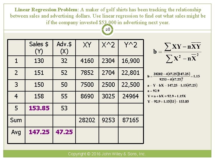
Linear Regression Problem: A maker of golf shirts has been tracking the relationship between sales and advertising dollars. Use linear regression to find out what sales might be if the company invested $53, 000 in advertising next year. 28 Sales $ (Y) Adv. $ (X) XY X^2 Y^2 1 130 32 4160 2304 16, 900 2 151 52 7852 2704 22, 801 3 150 50 7500 22, 500 4 158 55 8690 3025 24964 5 153. 85 53 28202 9253 87165 Sum Avg 147. 25 Copyright © 2016 John Wiley & Sons, Inc.

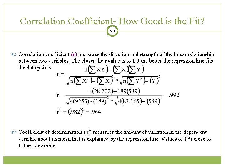
Correlation Coefficient- How Good is the Fit? 29 Correlation coefficient (r) measures the direction and strength of the linear relationship between two variables. The closer the r value is to 1. 0 the better the regression line fits the data points. Coefficient of determination ( ) measures the amount of variation in the dependent variable about its mean that is explained by the regression line. Values of ( ) close to 1. 0 are desirable.

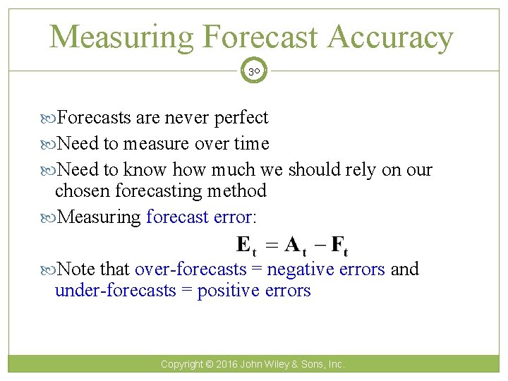
Measuring Forecast Accuracy 30 Forecasts are never perfect Need to measure over time Need to know how much we should rely on our chosen forecasting method Measuring forecast error: Note that over-forecasts = negative errors and under-forecasts = positive errors Copyright © 2016 John Wiley & Sons, Inc.

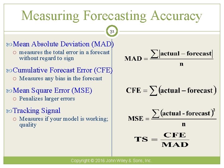
Measuring Forecasting Accuracy 31 Mean Absolute Deviation (MAD) measures the total error in a forecast without regard to sign Cumulative Forecast Error (CFE) Measures any bias in the forecast Mean Square Error (MSE) Penalizes larger errors Tracking Signal Measures if your model is working; quality Copyright © 2016 John Wiley & Sons, Inc.

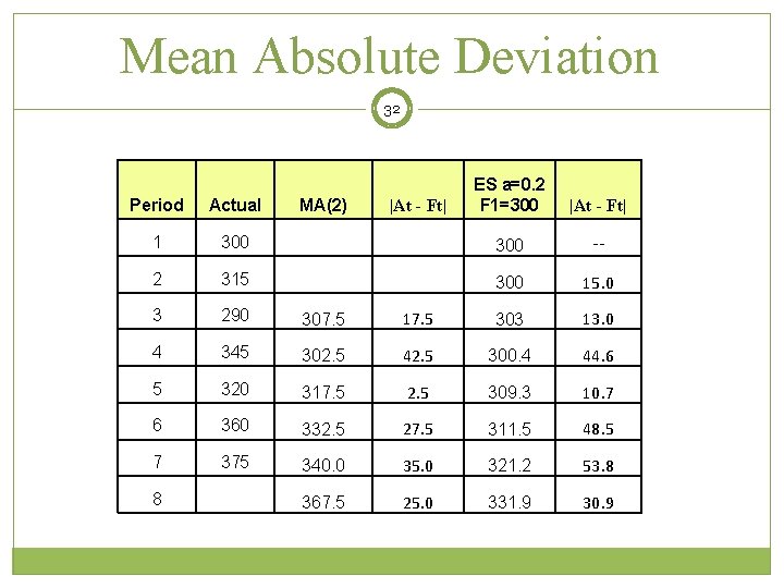
Mean Absolute Deviation 32 |At - Ft| Period Actual 1 300 -- 2 315 300 15. 0 3 290 307. 5 17. 5 303 13. 0 4 345 302. 5 42. 5 300. 4 44. 6 5 320 317. 5 2. 5 309. 3 10. 7 6 360 332. 5 27. 5 311. 5 48. 5 7 375 340. 0 35. 0 321. 2 53. 8 367. 5 25. 0 331. 9 30. 9 8 MA(2) ES a=0. 2 F 1=300 |At - Ft|

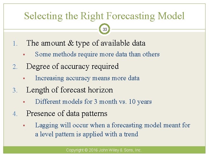
Selecting the Right Forecasting Model 33 The amount & type of available data 1. § Some methods require more data than others Degree of accuracy required 2. § Increasing accuracy means more data Length of forecast horizon 3. § Different models for 3 month vs. 10 years Presence of data patterns 4. § Lagging will occur when a forecasting model meant for a level pattern is applied with a trend Copyright © 2016 John Wiley & Sons, Inc.

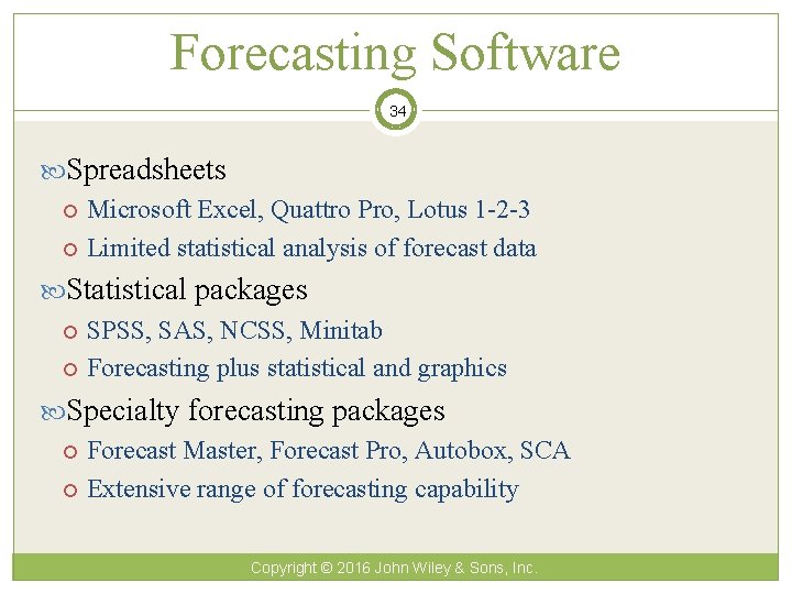
Forecasting Software 34 Spreadsheets Microsoft Excel, Quattro Pro, Lotus 1 -2 -3 Limited statistical analysis of forecast data Statistical packages SPSS, SAS, NCSS, Minitab Forecasting plus statistical and graphics Specialty forecasting packages Forecast Master, Forecast Pro, Autobox, SCA Extensive range of forecasting capability Copyright © 2016 John Wiley & Sons, Inc.

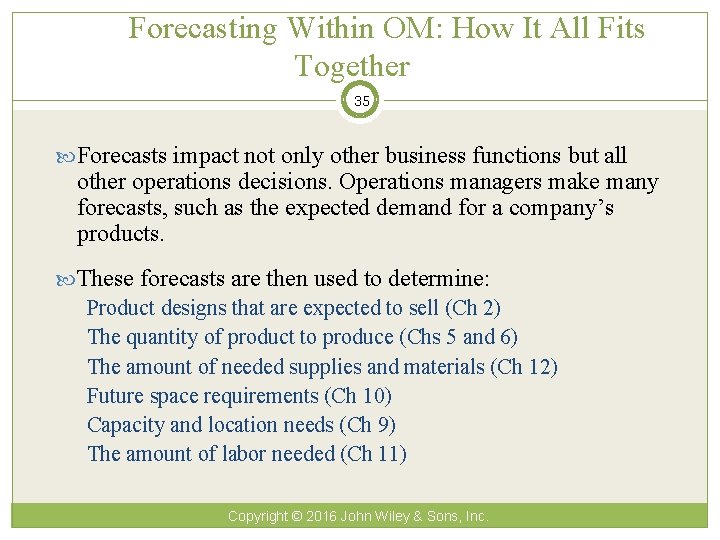
Forecasting Within OM: How It All Fits Together 35 Forecasts impact not only other business functions but all other operations decisions. Operations managers make many forecasts, such as the expected demand for a company’s products. These forecasts are then used to determine: Product designs that are expected to sell (Ch 2) The quantity of product to produce (Chs 5 and 6) The amount of needed supplies and materials (Ch 12) Future space requirements (Ch 10) Capacity and location needs (Ch 9) The amount of labor needed (Ch 11) Copyright © 2016 John Wiley & Sons, Inc.

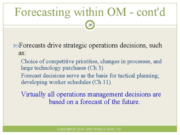
Forecasting within OM - cont'd 36 Forecasts drive strategic operations decisions, such as: Choice of competitive priorities, changes in processes, and large technology purchases (Ch 3) Forecast decisions serve as the basis for tactical planning; developing worker schedules (Ch 11) Virtually all operations management decisions are based on a forecast of the future. Copyright © 2016 John Wiley & Sons, Inc.

Forecasting Across the Organization 37 Forecasting is critical to management of all organizational functional areas Marketing relies on forecasting to predict demand future sales Finance forecasts stock prices, financial performance, capital investment needs. . Information systems provides ability to share databases and information Human resources forecasts future hiring requirements Copyright © 2016 John Wiley & Sons, Inc.

Chapter 8 Highlights 38 Three basic principles of forecasting are: forecasts are rarely perfect, are more accurate for groups than individual items, and are more accurate in the shorter term than longer time horizons. The forecasting process involves five steps: decide what to forecast, evaluate and analyze appropriate data, select and test model, generate forecast, and monitor accuracy. Forecasting methods can be classified into two groups: Qualitative methods are based on subjective opinion of forecaster and quantitative methods are based on mathematical modeling. Copyright © 2016 John Wiley & Sons, Inc.

Chapter 8 Highlights - cont'd 39 Time series models are based on the assumption that all information needed is contained in the time series of data. Causal models assume that the variable being forecast is related to other variables in the environment. There are four basic patterns of data: level or horizontal, trend, seasonality, and cycles. In addition, data usually contain random variation. Some forecast models used to forecast the level of a time series are: naïve, simple mean, simple moving average, weighted moving average, and exponential smoothing. Separate models are used to forecast trends and seasonality. Copyright © 2016 John Wiley & Sons, Inc.

Chapter 8 Highlights - cont'd 40 A simple causal model is linear regression in which a straight-line relationship is modeled between the variable we are forecasting and another variable in the environment. The correlation measures the strength of the linear relationship between these two variables. Three useful measures of forecast error are mean absolute deviation (MAD), mean square error (MSE) and tracking signal. There are four factors when selecting a model: amount and type of data available, degree of accuracy required, length of forecast horizon, and patterns present in the data. Copyright © 2016 John Wiley & Sons, Inc.