Chapter 8 Approximation Theory Given x 1 xm

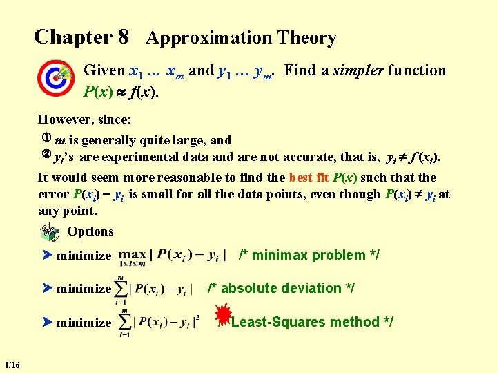
Chapter 8 Approximation Theory Given x 1 … xm and y 1 … ym. Find a simpler function P(x) f(x). However, since: ① m is generally quite large, and ② y ’s are experimental data and are not accurate, that is, y f (x ). i i i It would seem more reasonable to find the best fit P(x) such that the error P(xi) yi is small for all the data points, even though P(xi) yi at any point. Options minimize 1/16 /* minimax problem */ /* absolute deviation */ /* Least-Squares method */

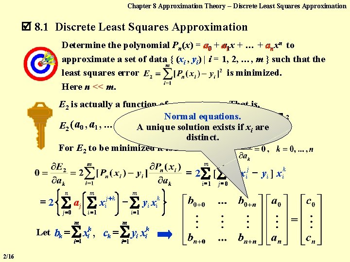
Chapter 8 Approximation Theory -- Discrete Least Squares Approximation 8. 1 Discrete Least Squares Approximation Determine the polynomial Pn(x) = a 0 + aa 11 x + … + anxn to approximate a set of data { (xi , yi) | i = 1, 2, …, m } such that the least squares error is minimized. Here n << m. E 2 is actually a function of a 0, a 1, …, an. That is, m Normal equations. n 2 + a 1 x i +exists yi. a 0 solution. . . + aifn xxii are E 2 ( a 0 , a 1 , . . . , a n ) = A unique = i 1 distinct. For E 2 to be minimized it is necessary that [ ] =2 m [ i =1 =2 n m j =0 aj Let bk = 2/16 m i =1 x j+k i m i =1 m yi xik k = x , c y x i i k i =1 k i i =1 n j=0 a j x ij y i ] x ik

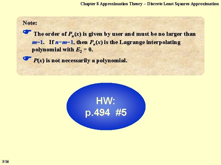
Chapter 8 Approximation Theory -- Discrete Least Squares Approximation Note: The order of Pn(x) is given by user and must be no larger than m 1. If n=m 1, then Pn(x) is the Lagrange interpolating polynomial with E 2 = 0. P(x) is not necessarily a polynomial. HW: p. 494 #5 3/16

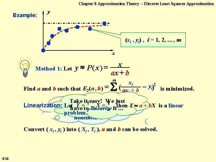
Chapter 8 Approximation Theory -- Discrete Least Squares Approximation Example: y (xi , yi) , i = 1, 2, …, m x Method 1: Let y P( x) = x ax + b m Find a and b such that E 2( a , b ) = i =1 xi ( ax + b i yi)2 is minimized. Take it easy! Weofjust But hey, the system Linearization: Lethave to linearize it , then Y a + b. X is a linear … equations for a and b is problem. nonlinear ! Convert ( xi , yi ) into ( Xi , Yi ), a and b can be solved. 4/16

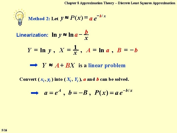
Chapter 8 Approximation Theory -- Discrete Least Squares Approximation Method 2: Let Linearization: y P( x) = a e b / x ln y ln a b x Y = ln y , X = x 1 , A = ln a , B = b Y A + BX is a linear problem Convert ( xi , yi ) into ( Xi , Yi ), a and b can be solved. 5/16

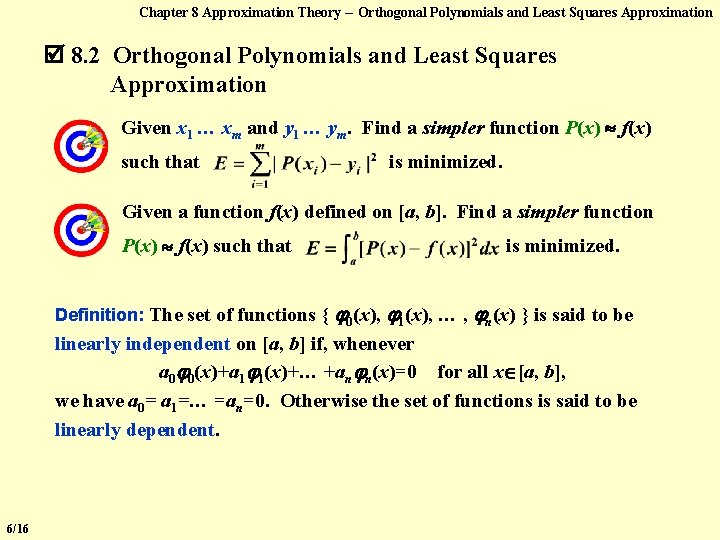
Chapter 8 Approximation Theory -- Orthogonal Polynomials and Least Squares Approximation 8. 2 Orthogonal Polynomials and Least Squares Approximation Given x 1 … xm and y 1 … ym. Find a simpler function P(x) f(x) such that is minimized. Given a function f(x) defined on [a, b]. Find a simpler function P(x) f(x) such that is minimized. Definition: The set of functions { 0(x), 1(x), … , n(x) } is said to be linearly independent on [a, b] if, whenever a 0 0(x)+a 1 1(x)+… +an n(x)=0 for all x [a, b], we have a 0= a 1=… =an=0. Otherwise the set of functions is said to be linearly dependent. 6/16

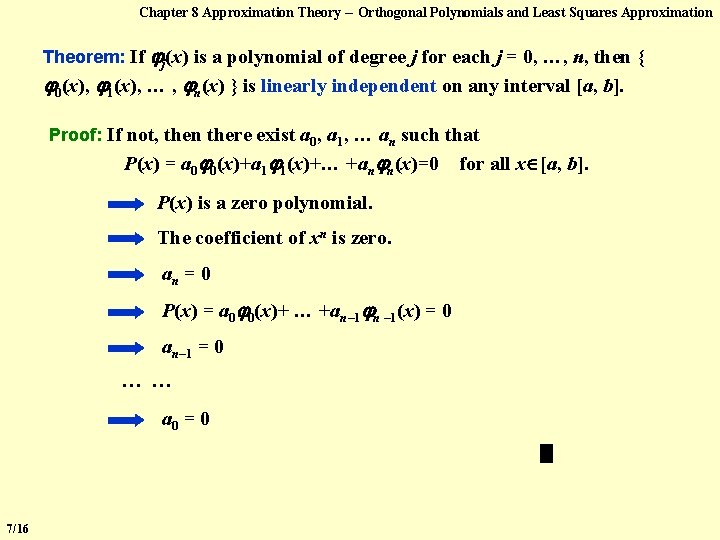
Chapter 8 Approximation Theory -- Orthogonal Polynomials and Least Squares Approximation Theorem: If j(x) is a polynomial of degree j for each j = 0, …, n, then { 0(x), 1(x), … , n(x) } is linearly independent on any interval [a, b]. Proof: If not, then there exist a 0, a 1, … an such that P(x) = a 0 0(x)+a 1 1(x)+… +an n(x)=0 P(x) is a zero polynomial. The coefficient of xn is zero. an = 0 P(x) = a 0 0(x)+ … +an– 1 n – 1(x) = 0 an– 1 = 0 …… a 0 = 0 7/16 for all x [a, b].

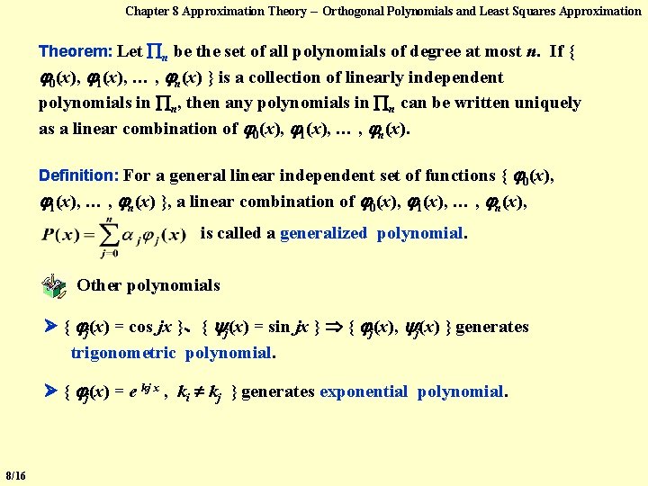
Chapter 8 Approximation Theory -- Orthogonal Polynomials and Least Squares Approximation Theorem: Let n be the set of all polynomials of degree at most n. If { 0(x), 1(x), … , n(x) } is a collection of linearly independent polynomials in n, then any polynomials in n can be written uniquely as a linear combination of 0(x), 1(x), … , n(x). Definition: For a general linear independent set of functions { 0(x), 1(x), … , n(x) }, a linear combination of 0(x), 1(x), … , n(x), is called a generalized polynomial. Other polynomials { j(x) = cos jx }、{ j(x) = sin jx } { j(x), j(x) } generates trigonometric polynomial. { j(x) = e kj x , ki kj } generates exponential polynomial. 8/16

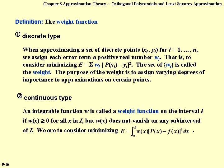
Chapter 8 Approximation Theory -- Orthogonal Polynomials and Least Squares Approximation Definition: The weight function ① discrete type When approximating a set of discrete points (xi , yi) for i = 1, …, n, we assign each error term a positive real number wi. That is, to consider minimizing E = wi [ P(xi) – yi]2. The set of {wi} is called the weight. The purpose of the weight is to assign varying degrees of importance to approximations on certain points. ② continuous type An integrable function w is called a weight function on the interval I if w(x) 0 for all x in I, but w(x) does not vanish on any subinterval of I. We are to consider minimizing 9/16 .

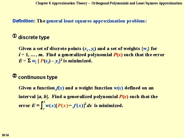
Chapter 8 Approximation Theory -- Orthogonal Polynomials and Least Squares Approximation Definition: The general least squares approximation problem: ① discrete type Given a set of discrete points (xi , yi) and a set of weights {wi} for i = 1, …, m. Find a generalized polynomial P(x) such that the error E = wi [ P(xi) – yi]2 is minimized. ② continuous type Given a function f(x) and a weight function w(x) defined on an interval [a, b]. Find a generalized polynomial P(x) such that the b error E = a w( x )[ P ( x ) f ( x )]2 dx is minimized. 10/16

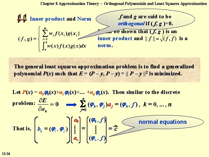
Chapter 8 Approximation Theory -- Orthogonal Polynomials and Least Squares Approximation f and g are said to be orthogonal if ( f, g )=0. It can be shown that ( f, g ) is an inner product and is a norm. Inner product and Norm The general least squares approximation problem is to find a generalized polynomial P(x) such that E = (P – y, P – y) = || P – y ||2 is minimized. Let P(x) = a 0 0(x)+a 1 1(x)+… +an n(x). Then similar to the discrete n ( problem: j =0 bij = ( i , j ) = an 11/16 , j )a j = ( k , f ) , k = 0, . . . , n ( 0 , f ) a 0 That is, k =c ( n , f ) normal equations

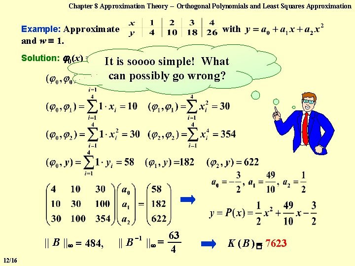
Chapter 8 Approximation Theory -- Orthogonal Polynomials and Least Squares Approximation Example: Approximate with and w 1. 2 Solution: 0(x) = 1，It is = x， (x) = x 1(x) 2 soooo simple! What can possibly go wrong? || B || = 484, 12/16 || B 1 || = 63 4 K ( B )� = 7623

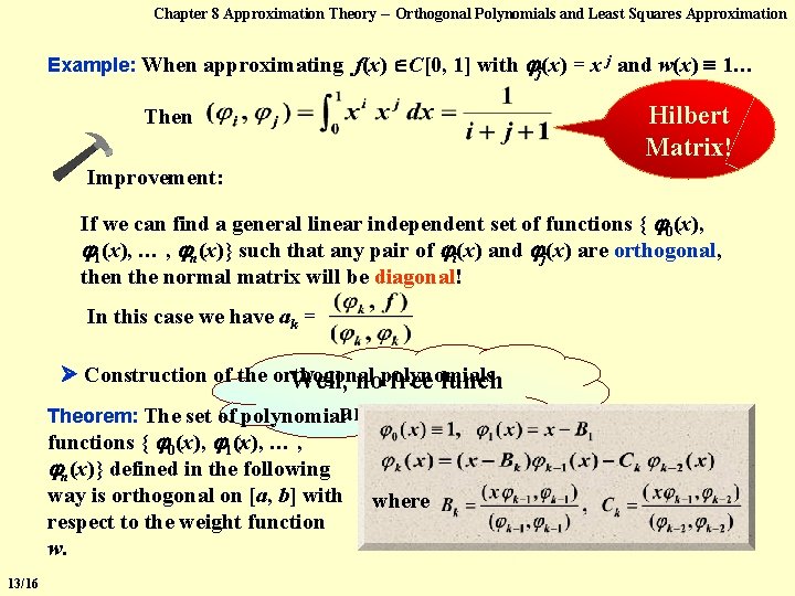
Chapter 8 Approximation Theory -- Orthogonal Polynomials and Least Squares Approximation Example: When approximating f(x) C[0, 1] with j(x) = x j and w(x) 1… Hilbert Matrix! Then Improvement: If we can find a general linear independent set of functions { 0(x), 1(x), … , n(x)} such that any pair of i(x) and j(x) are orthogonal, then the normal matrix will be diagonal! In this case we have ak = Construction of the orthogonal Well, nopolynomials free lunch Theorem: The set of polynomialanyway… functions { 0(x), 1(x), … , n(x)} defined in the following way is orthogonal on [a, b] with respect to the weight function w. 13/16 where

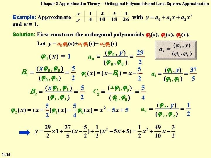
Chapter 8 Approximation Theory -- Orthogonal Polynomials and Least Squares Approximation Example: Approximate with and w 1. Solution: First construct the orthogonal polynomials 0(x), 1(x), 2(x). Let y = a 0 0(x)+a 1 1(x)+ a 2 2(x) ( 0 , y ) 29 = ( 0 , 0 ) 2 ( x 0 , 0 ) 5 5 ( 1 , y ) 37 B 1 = = 1 ( x ) = ( x B 1 ) = x = a 1 = ( 0, 0) 2 2 ( 1 , 1 ) 5 ( x 1, 0 ) 5 C 2 = B 2 = = = ( 1 , 1 ) 2 ( 0 , 0 ) 4 ( 2 , y ) 1 5 5 2 = = a 2 ( x ) = ( x ) 1 ( x ) 0 ( x ) = x 5 x + 5 2 ( 2 , 2 ) 2 2 4 0( x) = 1 14/16 a 0 =

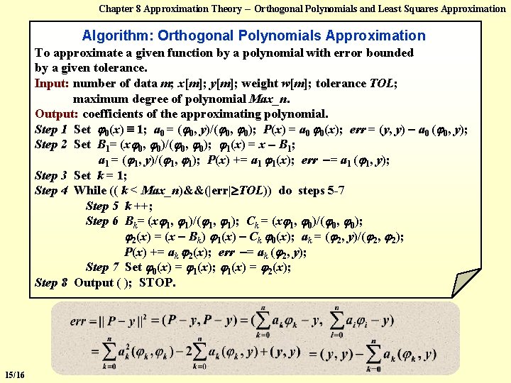
Chapter 8 Approximation Theory -- Orthogonal Polynomials and Least Squares Approximation Algorithm: Orthogonal Polynomials Approximation To approximate a given function by a polynomial with error bounded by a given tolerance. Input: number of data m; x[m]; y[m]; weight w[m]; tolerance TOL; maximum degree of polynomial Max_n. Output: coefficients of the approximating polynomial. Step 1 Set 0(x) 1; a 0 = ( 0, y)/( 0, 0); P(x) = a 0 0(x); err = (y, y) a 0 ( 0, y); Step 2 Set B 1= (x 0, 0)/( 0, 0); 1(x) = x B 1; a 1 = ( 1, y)/( 1, 1); P(x) += a 1 1(x); err = a 1 ( 1, y); Step 3 Set k = 1; Step 4 While (( k < Max_n)&&(|err| TOL)) do steps 5 -7 Step 5 k ++; Step 6 Bk= (x 1, 1)/( 1, 1); Ck = (x 1, 0)/( 0, 0); 2(x) = (x Bk) 1(x) Ck 0(x); ak = ( 2, y)/( 2, 2); P(x) += ak 2(x); err = ak ( 2, y); Step 7 Set 0(x) = 1(x); 1(x) = 2(x); Step 8 Output ( ); STOP. 15/16

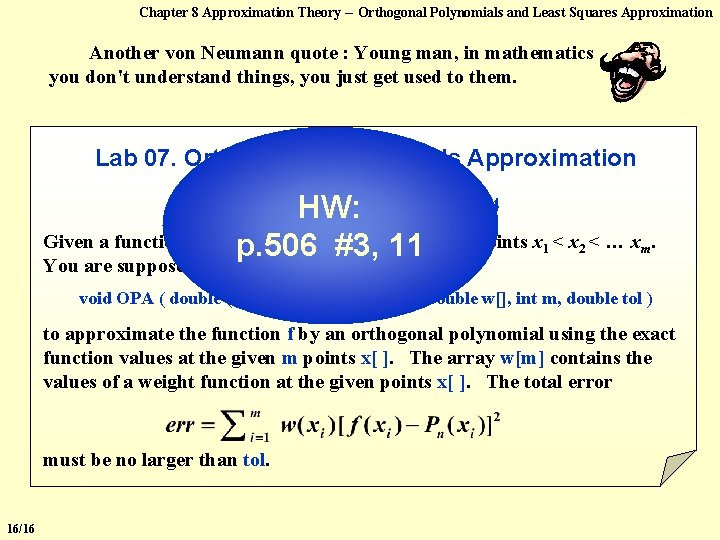
Chapter 8 Approximation Theory -- Orthogonal Polynomials and Least Squares Approximation Another von Neumann quote : Young man, in mathematics you don't understand things, you just get used to them. Lab 07. Orthogonal Polynomials Approximation HW: Given a function f and p. 506 a set of 200 #3, m > 11 0 distinct points x 1 < x 2 < … xm. You are supposed to write a function Time Limit: 1 second; Points: 4 void OPA ( double (*f)(double x), double x[], double w[], int m, double tol ) to approximate the function f by an orthogonal polynomial using the exact function values at the given m points x[ ]. The array w[m] contains the values of a weight function at the given points x[ ]. The total error must be no larger than tol. 16/16